knitr::opts_chunk$set(echo = TRUE)
library(revolver)
Since the new release of REVOLVER (>= 0.3), we have
implemented all
plotting functions using ggplot2.
All functions now return either a ggplot object, or a
more complext figure obtained by assembling ggplot objects
either via ggarrange (package ggpubr)
or plot_grid (package cowplot)
cowplot. Notice that some functions might be only
applicable after fits or clusters have been computed (the package will
raise errors if you try to call a function on an object that does not
have the required information to create the plot).
In this vignette, we apply the plotting functions to one of the
cohort objects released in the evoverse.datasets R package.
# Data released in the 'evoverse.datasets'
data('TRACERx_NEJM_2017_REVOLVER', package = 'evoverse.datasets')
Plotting cohort-level data
You can plot various information about the drivers in the cohort, and the trajectories detected in the cohort. See the manual of each one of these functions to understand non-trivial plots, and how to customize the input parameters.
# Plot the occurrence of drivers across the cohort.
plot_drivers_occurrence(TRACERx_NEJM_2017_REVOLVER)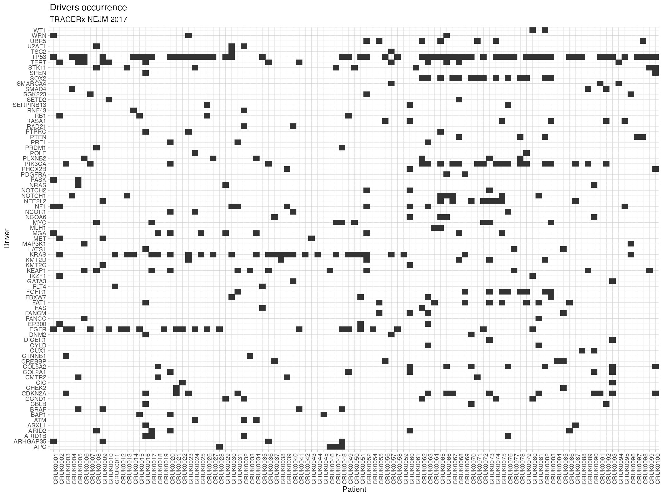
# Plot the barplot of drivers' occurrences (clonal vs subclonal)
plot_drivers_clonality(TRACERx_NEJM_2017_REVOLVER) 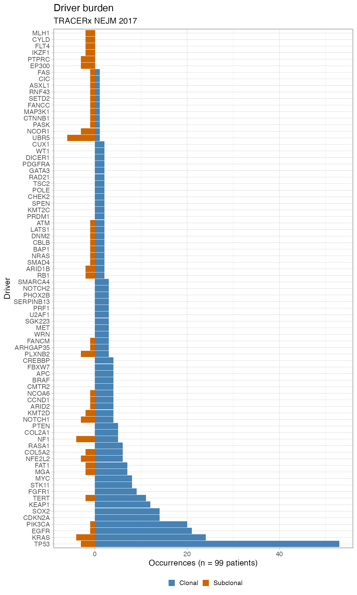
# Plot the  graph-alike summary statistics for the cohort drivers.
plot_drivers_graph(TRACERx_NEJM_2017_REVOLVER)
#>
#> =-=-=-=-=-=-=-=-=-=-=-=-=-=-=-=-=-=-
#>  Enrichment test for incoming edges
#> =-=-=-=-=-=-=-=-=-=-=-=-=-=-=-=-=-=-
#> # A tibble: 49 × 15
#>    estimate    p.value conf.low conf.high method alternative from  to    POS_POS
#>       <dbl>      <dbl>    <dbl>     <dbl> <chr>  <chr>       <chr> <chr>   <int>
#>  1     23.0    1.82e-9     8.60       Inf Fishe… greater     EGFR  TP53       13
#>  2     25.4    1.36e-6     4.81       Inf Fishe… greater     GL    PIK3…      20
#>  3     10.5    6.27e-6     4.19       Inf Fishe… greater     CDKN… TP53       10
#>  4     12.6    8.68e-6     3.56       Inf Fishe… greater     GL    EGFR       20
#>  5    Inf      1.48e-5     5.16       Inf Fishe… greater     GL    CDKN…      14
#>  6    Inf      1.48e-5     5.16       Inf Fishe… greater     GL    SOX2       14
#>  7     19.8    1.71e-5     5.37       Inf Fishe… greater     TP53  FAT1        7
#>  8    Inf      2.10e-5     9.42       Inf Fishe… greater     RASA1 TP53        5
#>  9    Inf      5.99e-5    14.5        Inf Fishe… greater     BRAF  TERT        3
#> 10    Inf      7.41e-5     4.31       Inf Fishe… greater     GL    KEAP1      12
#> # ℹ 39 more rows
#> # ℹ 6 more variables: POS_NEG <int>, NEG_POS <int>, NEG_NEG <int>,
#> #   alpha_level <dbl>, N <int>, psign <lgl>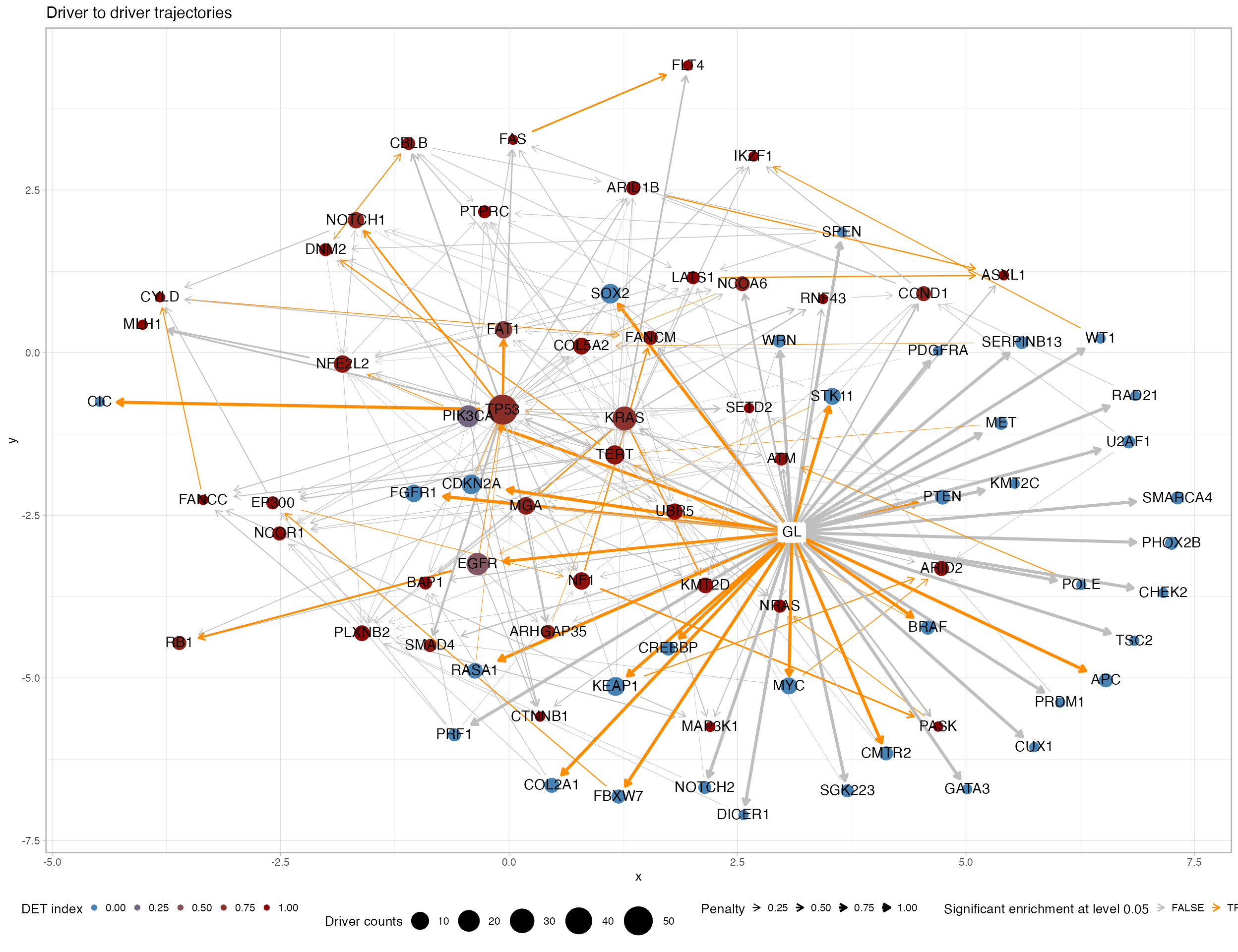
This graph plot can be simplified reduce the entries used to generate
the edges - try for instance using min.occurrences = 5.
You can also plot the penalty of the fit, and the DET index derived from that
# Plot the index of Divergent Evolutionary Trajectories
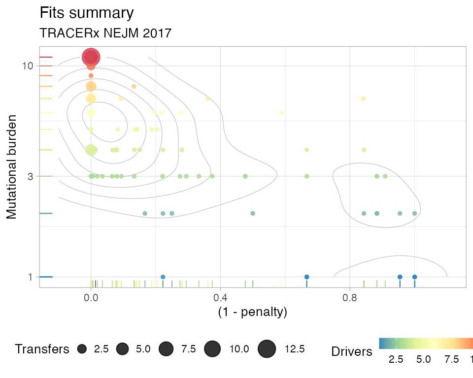
plot_penalty(TRACERx_NEJM_2017_REVOLVER)
#>
#> =-=-=-=-=-=-=-=-=-=-=-=-=-=-=-=-=-=-
#>  Enrichment test for incoming edges
#> =-=-=-=-=-=-=-=-=-=-=-=-=-=-=-=-=-=-
#> # A tibble: 49 × 15
#>    estimate    p.value conf.low conf.high method alternative from  to    POS_POS
#>       <dbl>      <dbl>    <dbl>     <dbl> <chr>  <chr>       <chr> <chr>   <int>
#>  1     23.0    1.82e-9     8.60       Inf Fishe… greater     EGFR  TP53       13
#>  2     25.4    1.36e-6     4.81       Inf Fishe… greater     GL    PIK3…      20
#>  3     10.5    6.27e-6     4.19       Inf Fishe… greater     CDKN… TP53       10
#>  4     12.6    8.68e-6     3.56       Inf Fishe… greater     GL    EGFR       20
#>  5    Inf      1.48e-5     5.16       Inf Fishe… greater     GL    CDKN…      14
#>  6    Inf      1.48e-5     5.16       Inf Fishe… greater     GL    SOX2       14
#>  7     19.8    1.71e-5     5.37       Inf Fishe… greater     TP53  FAT1        7
#>  8    Inf      2.10e-5     9.42       Inf Fishe… greater     RASA1 TP53        5
#>  9    Inf      5.99e-5    14.5        Inf Fishe… greater     BRAF  TERT        3
#> 10    Inf      7.41e-5     4.31       Inf Fishe… greater     GL    KEAP1      12
#> # ℹ 39 more rows
#> # ℹ 6 more variables: POS_NEG <int>, NEG_POS <int>, NEG_NEG <int>,
#> #   alpha_level <dbl>, N <int>, psign <lgl>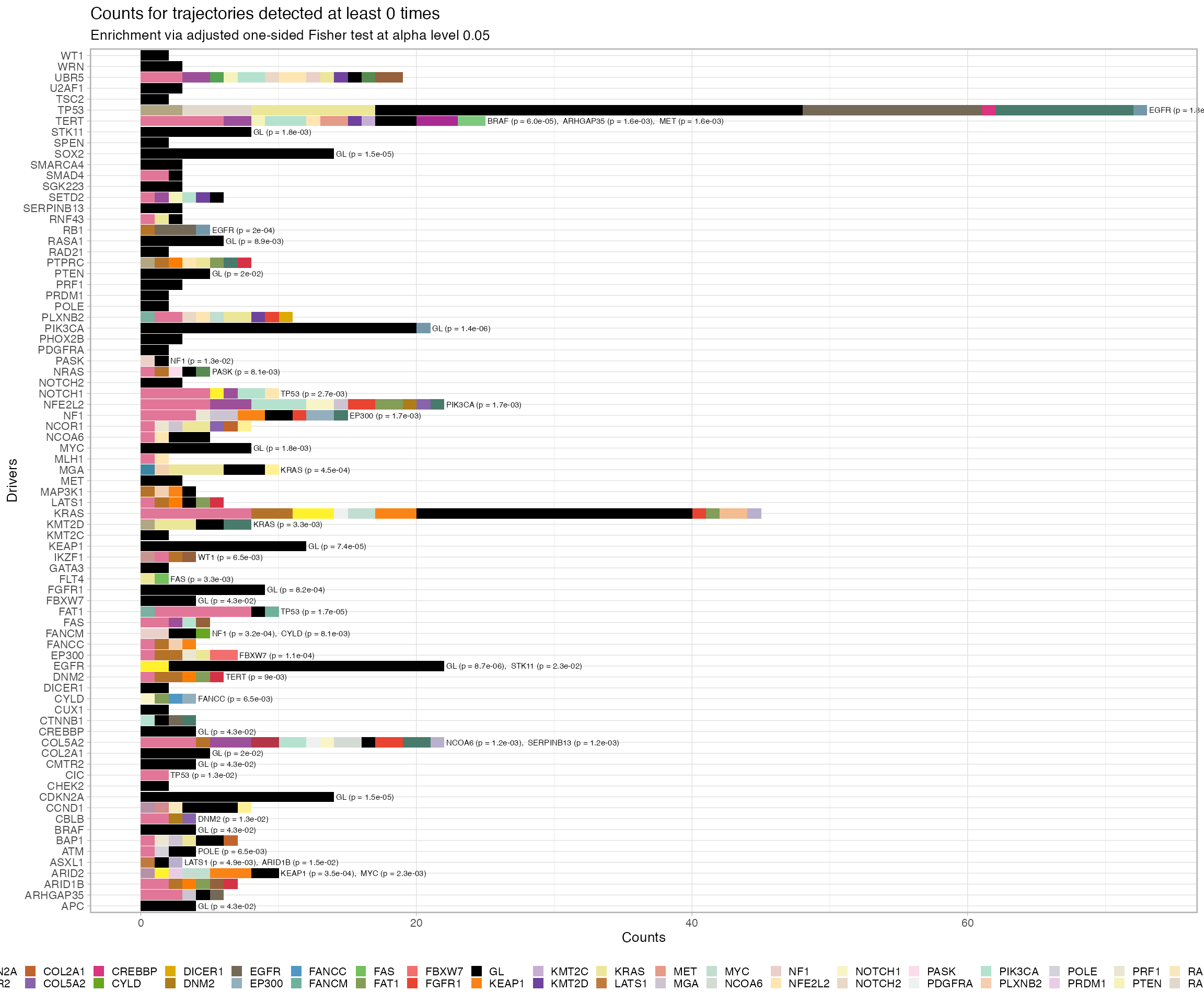
# Plot the index of Divergent Evolutionary Trajectories
plot_DET_index(TRACERx_NEJM_2017_REVOLVER)
#> # A tibble: 79 × 4
#>    driver diversity     N DET_index
#>    <chr>      <dbl> <int>     <dbl>
#>  1 APC            0     1         0
#>  2 BRAF           0     1         0
#>  3 CDKN2A         0     1         0
#>  4 CHEK2          0     1         0
#>  5 CIC            0     1         0
#>  6 CMTR2          0     1         0
#>  7 COL2A1         0     1         0
#>  8 CREBBP         0     1         0
#>  9 CUX1           0     1         0
#> 10 DICER1         0     1         0
#> # ℹ 69 more rows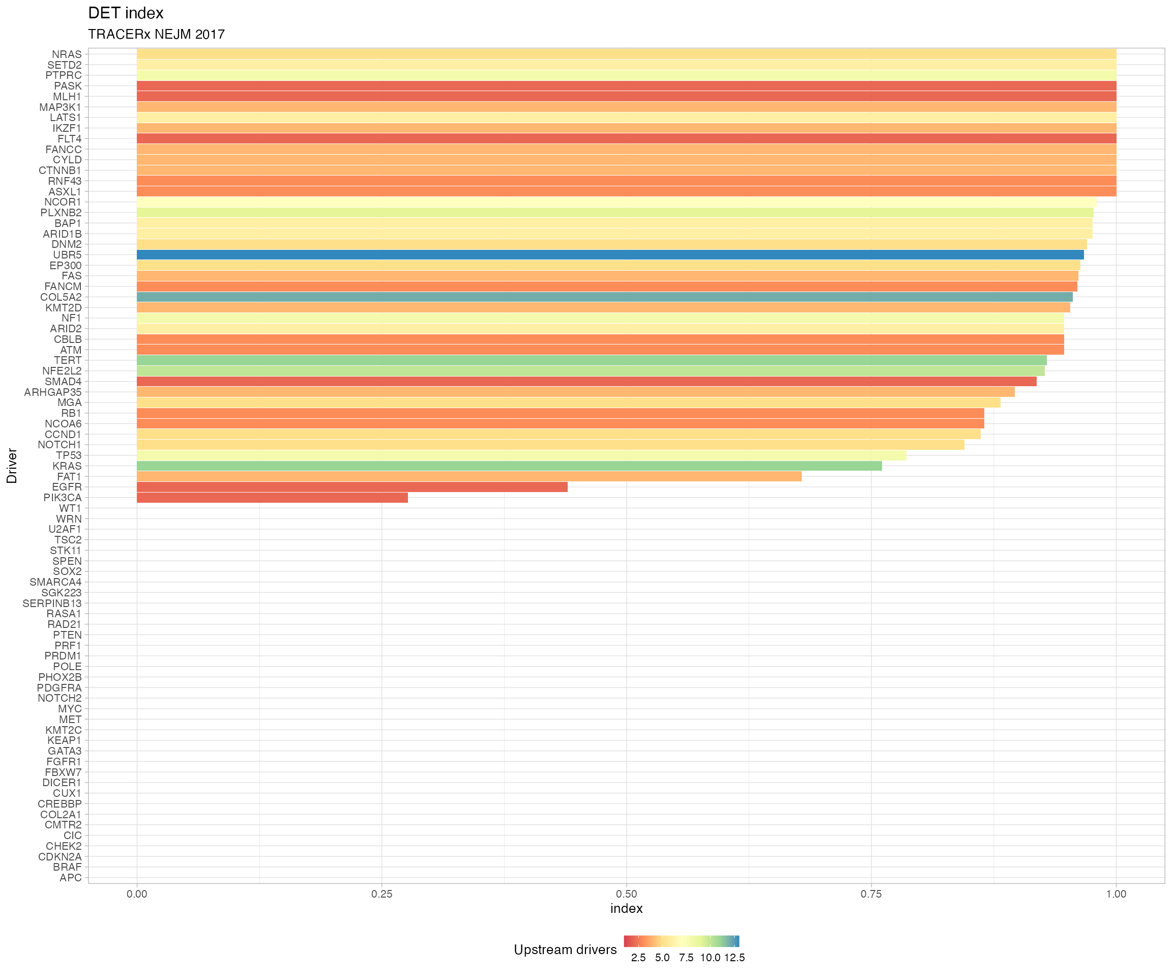
Plotting patient’s data and trees
You can plot the data and the trees of a patient.
# Plot the data histogram for a patient.
plot_patient_CCF_histogram(TRACERx_NEJM_2017_REVOLVER, 'CRUK0002')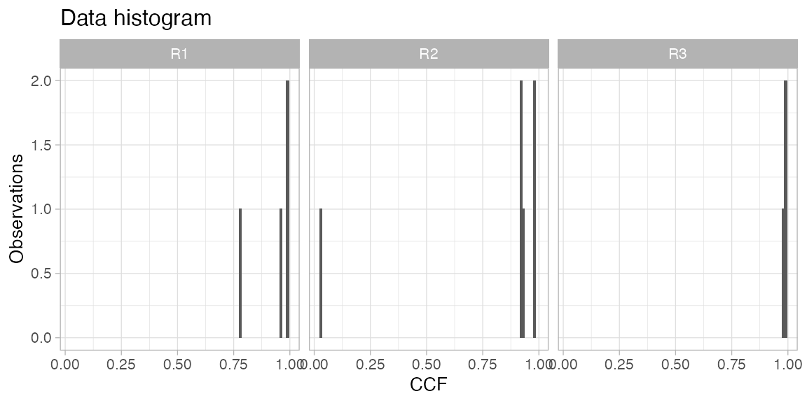
# Plot the mutation burden for a patient.
plot_patient_mutation_burden(TRACERx_NEJM_2017_REVOLVER, 'CRUK0002')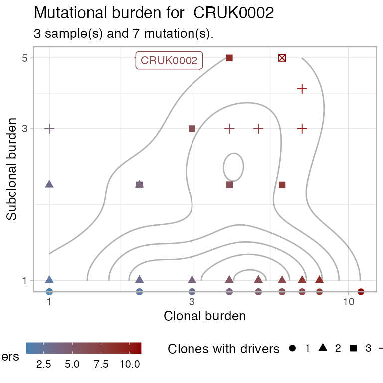
# Plot the oncoprint for a patient.
plot_patient_oncoprint(TRACERx_NEJM_2017_REVOLVER, 'CRUK0002')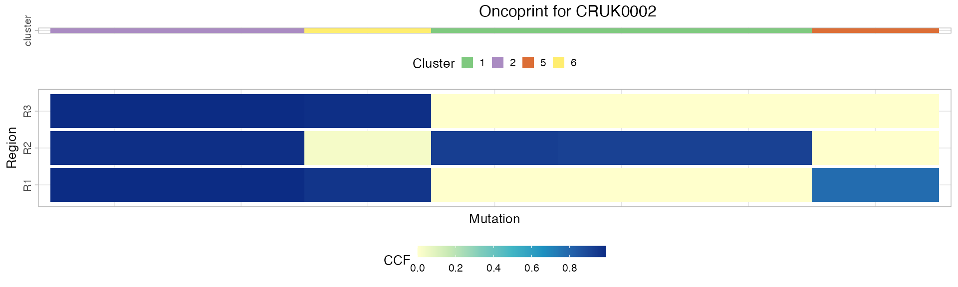
A full profile of the data available for a patient can be print using
plot_patient_data. This function uses the above functions
in combination with functions that are specific to the packages that
implements the trees of the current cohort, in order to create other
visualization of the data.
In the case of this cohort, since the patients have CCF-based clone trees, the reference plotting functions are from the ctree package
# Plot a number of different measurements for the patient
plot_patient_data(TRACERx_NEJM_2017_REVOLVER, 'CRUK0002')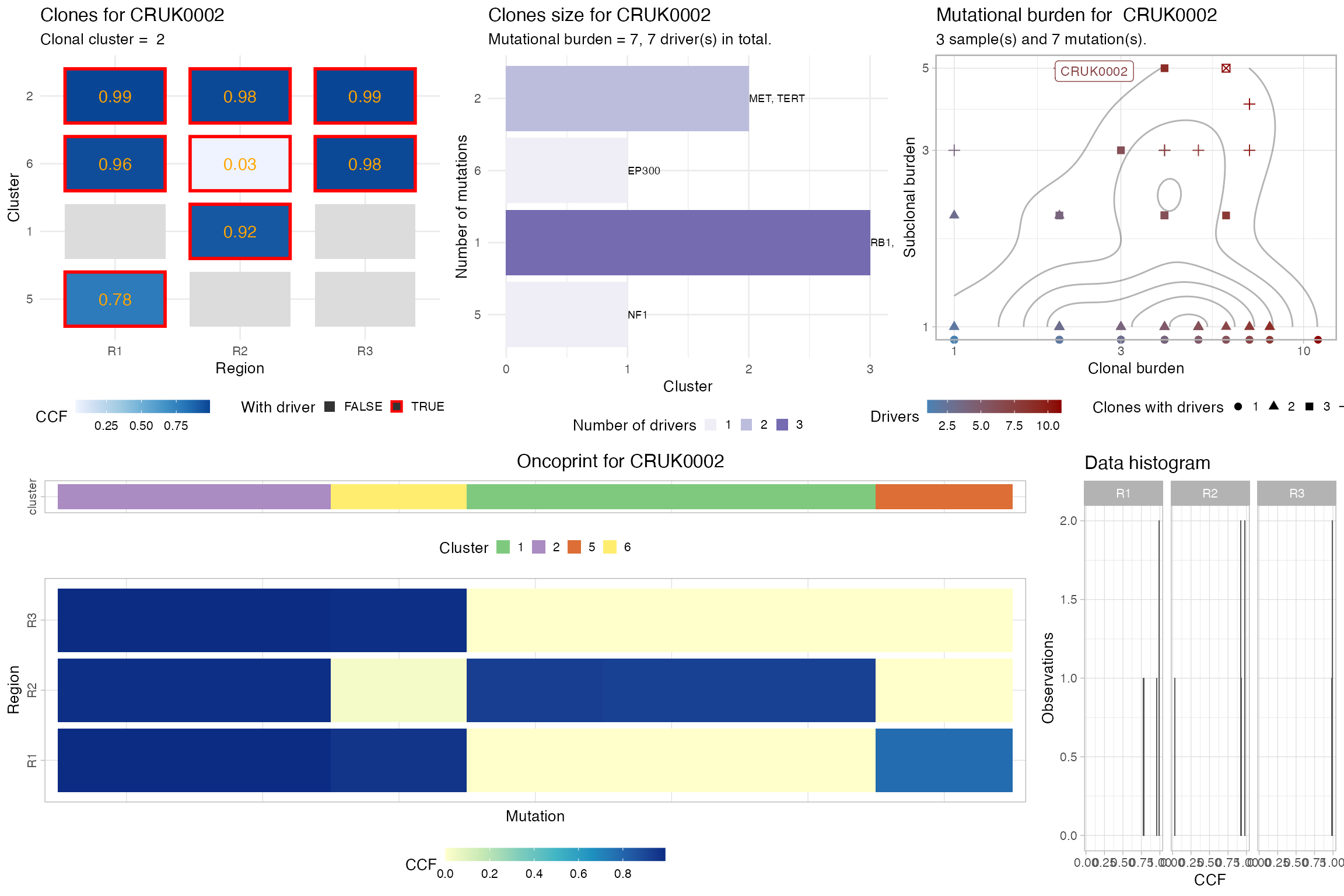
In a similar way, trees are plot using functions from the ctree package, called by
REVOLVER.
# Plot REVOLVER trees for a patient.
plot_patient_trees(TRACERx_NEJM_2017_REVOLVER, 'CRUK0002')
#> This graph was created by an old(er) igraph version.
#> ℹ Call `igraph::upgrade_graph()` on it to use with the current igraph version.
#> For now we convert it on the fly...
#> This graph was created by an old(er) igraph version.
#> ℹ Call `igraph::upgrade_graph()` on it to use with the current igraph version.
#> For now we convert it on the fly...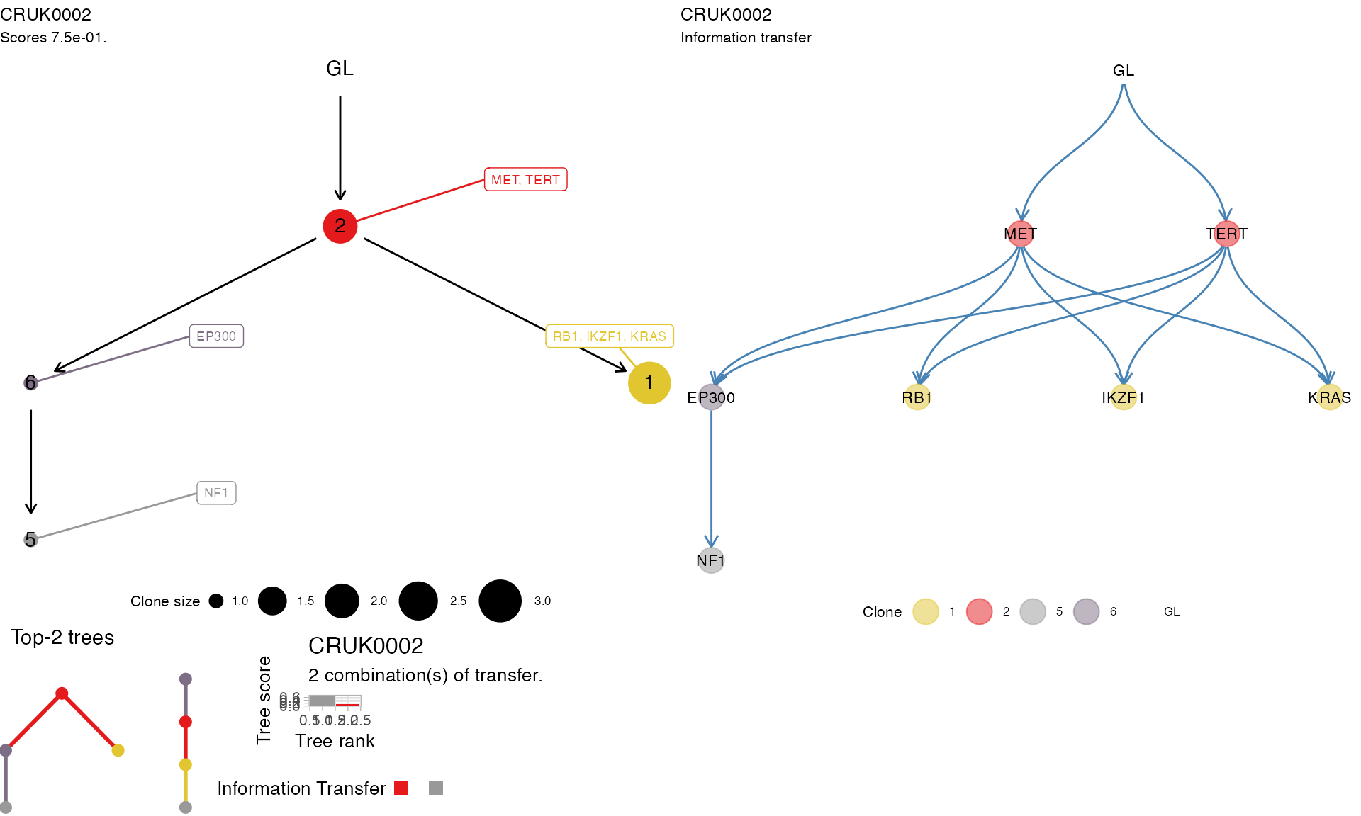
The above function plots the tree score as
# Plot REVOLVER trees for a patient.
plot_patient_trees_scores(TRACERx_NEJM_2017_REVOLVER, 'CRUK0002')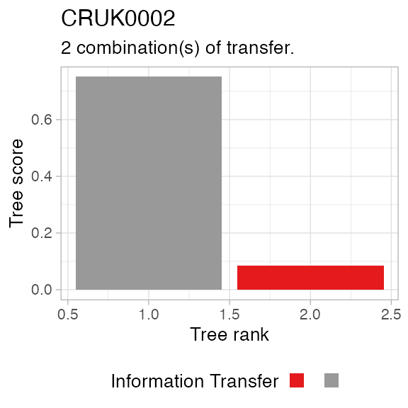
Plotting REVOLVER clusters and jackknife statistics
The results of using REVOLVER to cluster your cohort can
be visualised with two functions
# Plot the heatmaps of REVOLVER"s clusters, as tiles.
plot_clusters(TRACERx_NEJM_2017_REVOLVER)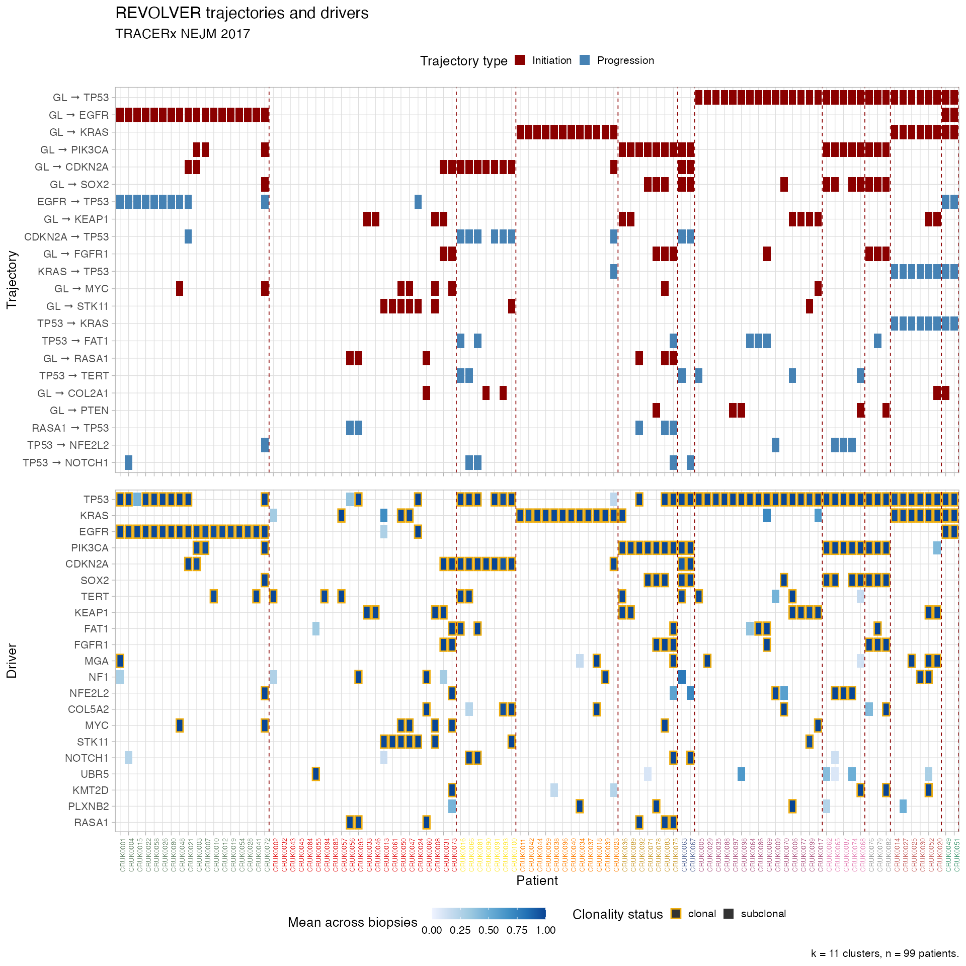
The top tile is patients vs trajectories, and bottom is patients vs drivers. For drivers colours reflect mean CCF/ binary values of a driver in every patient, and clonality status. For trajectories colours reflect if they are initiating or progressing, depending on the present of GL in the trajectory (GL stands for germline).
The dendrogram of the clusters can be visualised - notice the colours and patients’ ordering that are matched in these two functions.
# Plot the dendrogram of REVOLVER"s clusters
revolver::plot_dendrogram(TRACERx_NEJM_2017_REVOLVER)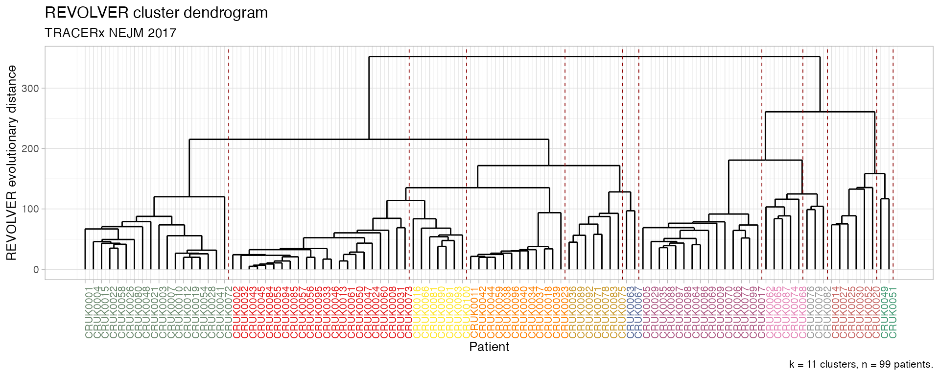
You can also compute the number of trajectories per cluster, and their frequency.
# Plot the trajectories detected in at least 10 patients per cluster
plot_trajectories_per_cluster(TRACERx_NEJM_2017_REVOLVER, min_counts = 10)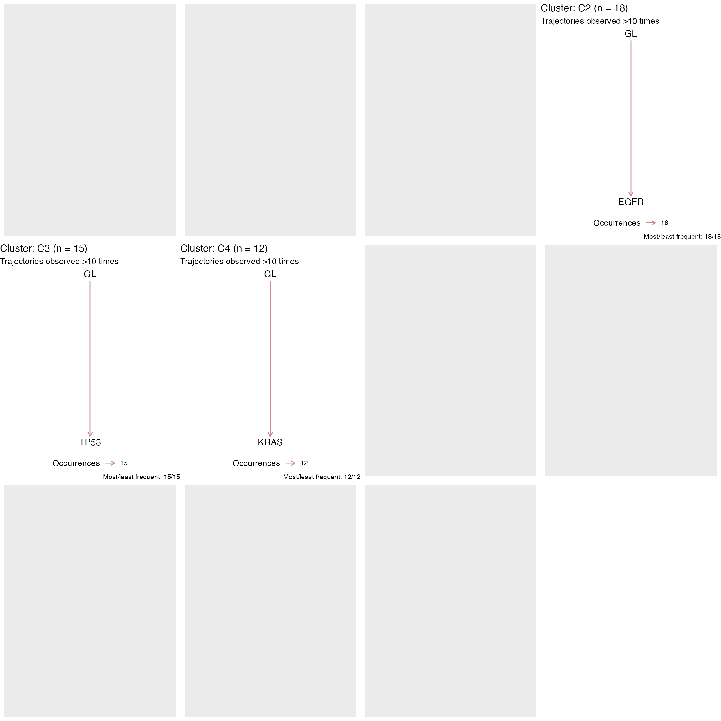
# Plot the trajectories detected in at least 30% patients per cluster
plot_trajectories_per_cluster(TRACERx_NEJM_2017_REVOLVER, min_counts = .3)
#> → min_counts in [0,1], interpreting that as a proportion.
#> → min_counts in [0,1], interpreting that as a proportion.
#> → min_counts in [0,1], interpreting that as a proportion.
#> → min_counts in [0,1], interpreting that as a proportion.
#> → min_counts in [0,1], interpreting that as a proportion.
#> → min_counts in [0,1], interpreting that as a proportion.
#> → min_counts in [0,1], interpreting that as a proportion.
#> → min_counts in [0,1], interpreting that as a proportion.
#> → min_counts in [0,1], interpreting that as a proportion.
#> → min_counts in [0,1], interpreting that as a proportion.
#> → min_counts in [0,1], interpreting that as a proportion.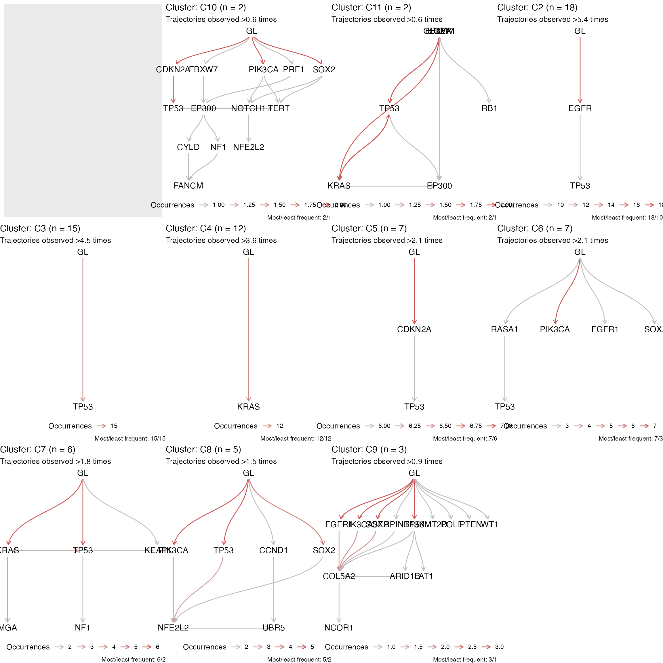
After jackknife, you can also plot the co-clustering probability of the patients, the clustering stability and other statistics about the trajectories.
# Plot the patients' jackknife co-clustering probability
plot_jackknife_coclustering(TRACERx_NEJM_2017_REVOLVER)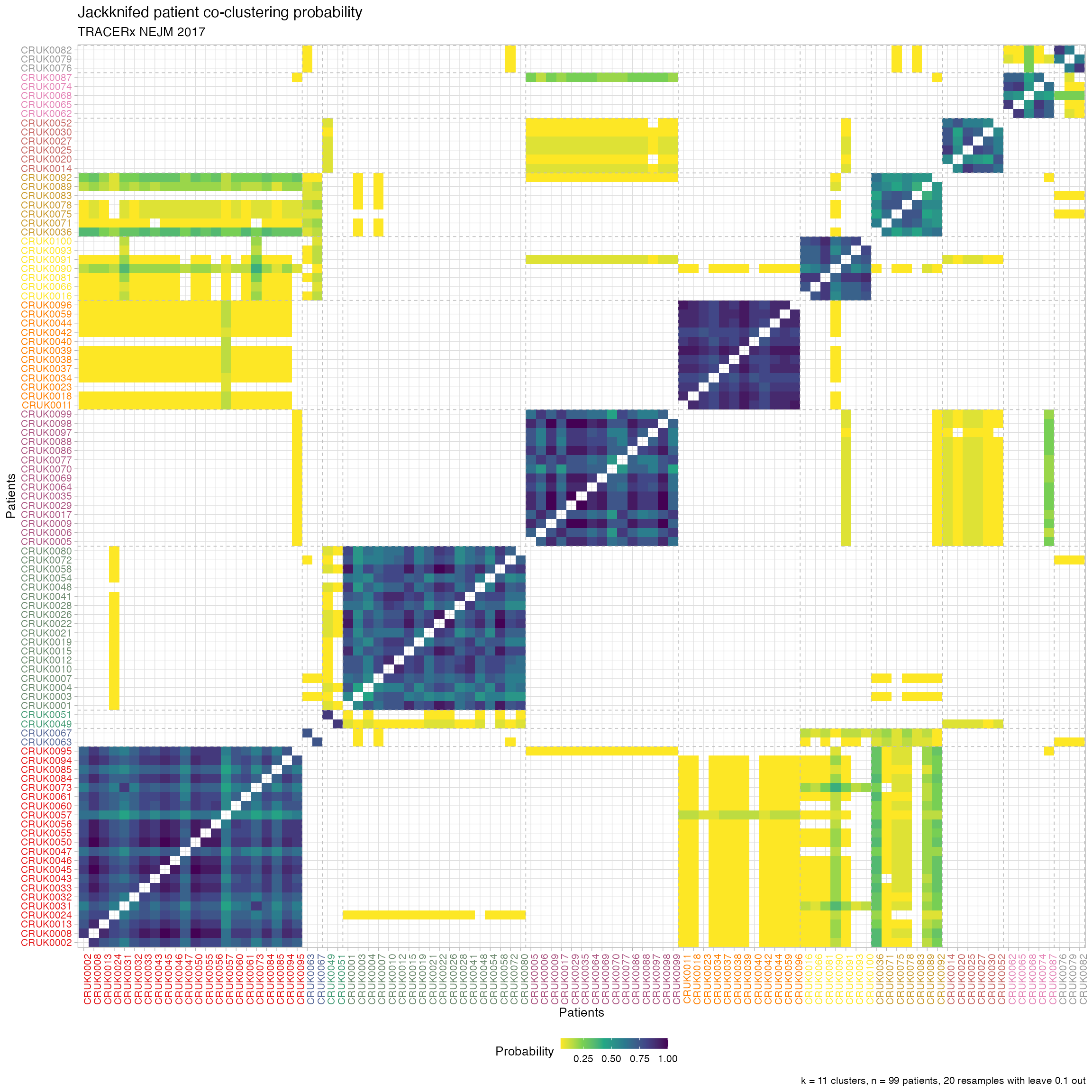
# Plot the patients' jackknife cluster staability
plot_jackknife_cluster_stability(TRACERx_NEJM_2017_REVOLVER)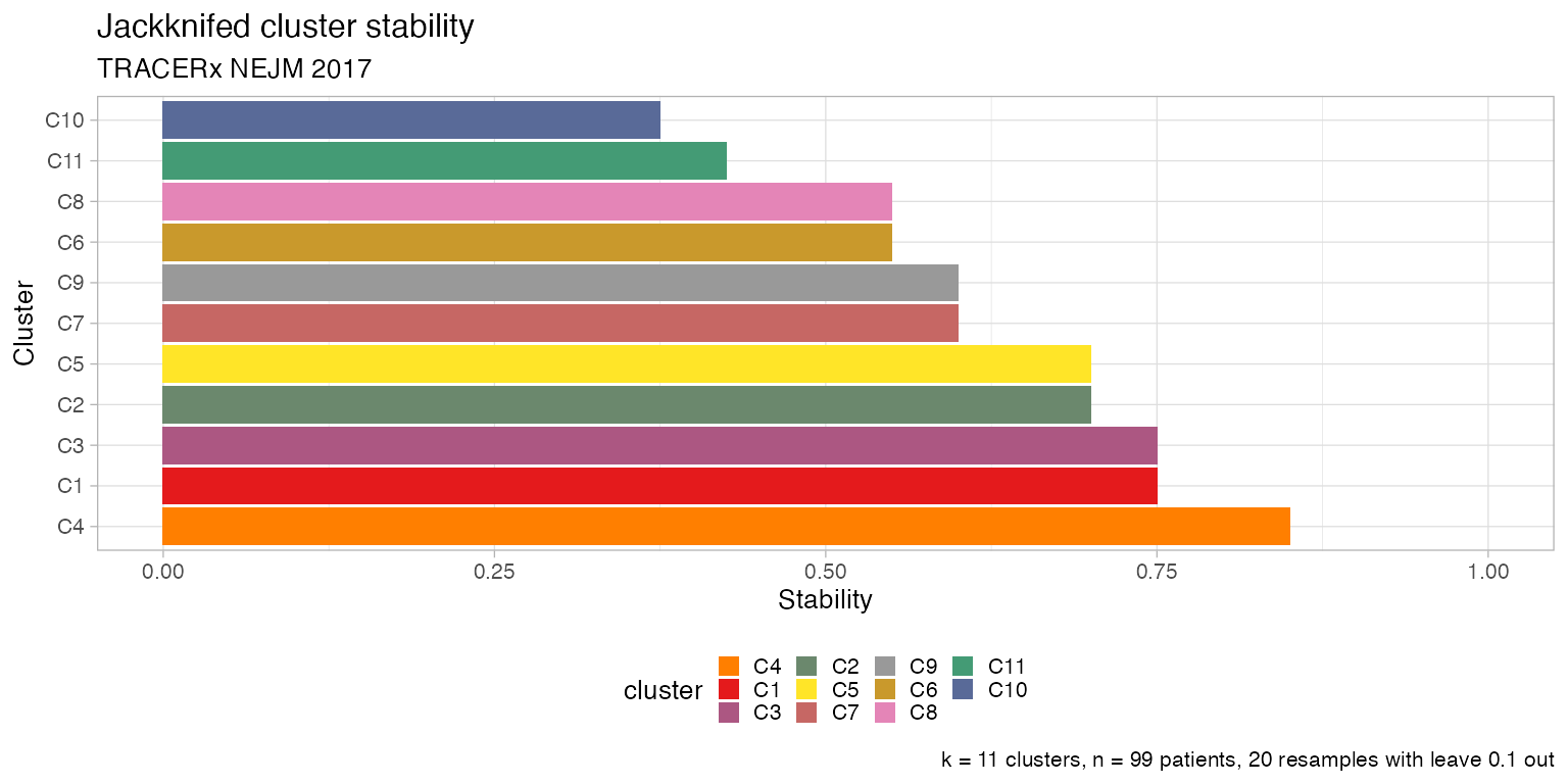
# Plot the patients' jackknife trajectory frequencies.
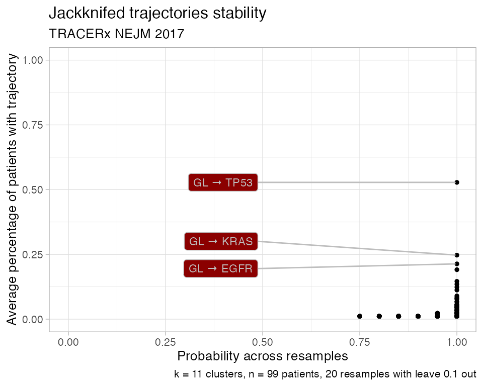
plot_jackknife_trajectories_stability(TRACERx_NEJM_2017_REVOLVER)