Plot graph-alike summary statistics for the cohort drivers.

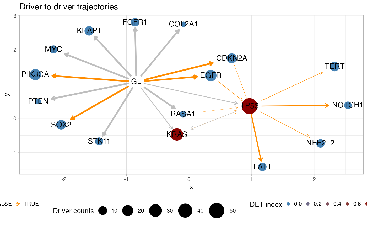
Plot a graph with driver genes and annotate with different summary statistics for the trajectories that involve the drivers. This visualisation shows the frequency of the driver in the cohort (node size), the penalty for each pair of odering (edge thickness), the significance for the pair of orderings as of a Fisher test (edge coloring) and the overall heterogeneity upstream a driver as of the DET index (node coloring). This function has parameters to subset the computation to a list of predefined drivers, or drivers associated to trajectories with a minimum recurrence in the fits.

plot_drivers_graph(
  x,
  drivers = x$variantIDs.driver,
  min.occurrences = 0,
  alpha_level = 0.05,
  ...
)

Arguments

x

A REVOLVER object with fits.

drivers

The list of drivers to consider, all by default. See also function plot_penalty.

min.occurrences

The minimum number of occurrences for a trajectory to be considered, zero by default. See also function plot_penalty.

alpha_level

The significance level for the enrichment Fisher test.

...

Extra parameters passed to the create_layout function by ggraph. For instance, passing algorithm = 'kk' and layout = 'igraph' the `igraph` layout `kk` will be adopted.

Value

A `ggplot` object of the plot.

See also

Other Plotting functions: distinct_palette_few(), distinct_palette_many(), gradient_palette(), plot_DET_index(), plot_clusters(), plot_dendrogram(), plot_drivers_clonality(), plot_drivers_occurrence(), plot_jackknife_cluster_stability(), plot_jackknife_coclustering(), plot_jackknife_trajectories_stability(), plot_patient_CCF_histogram(), plot_patient_data(), plot_patient_mutation_burden(), plot_patient_oncoprint(), plot_patient_trees_scores()

Examples

# Data released in the 'evoverse.datasets'
data('TRACERx_NEJM_2017_REVOLVER', package = 'evoverse.datasets')

# Base plot, can be quite crowded
plot_drivers_graph(TRACERx_NEJM_2017_REVOLVER)
#> 
#> =-=-=-=-=-=-=-=-=-=-=-=-=-=-=-=-=-=-
#>  Enrichment test for incoming edges
#> =-=-=-=-=-=-=-=-=-=-=-=-=-=-=-=-=-=-
#> # A tibble: 49 × 15
#>    estimate    p.value conf.low conf.high method alternative from  to    POS_POS
#>       <dbl>      <dbl>    <dbl>     <dbl> <chr>  <chr>       <chr> <chr>   <int>
#>  1     23.0    1.82e-9     8.60       Inf Fishe… greater     EGFR  TP53       13
#>  2     25.4    1.36e-6     4.81       Inf Fishe… greater     GL    PIK3…      20
#>  3     10.5    6.27e-6     4.19       Inf Fishe… greater     CDKN… TP53       10
#>  4     12.6    8.68e-6     3.56       Inf Fishe… greater     GL    EGFR       20
#>  5    Inf      1.48e-5     5.16       Inf Fishe… greater     GL    CDKN…      14
#>  6    Inf      1.48e-5     5.16       Inf Fishe… greater     GL    SOX2       14
#>  7     19.8    1.71e-5     5.37       Inf Fishe… greater     TP53  FAT1        7
#>  8    Inf      2.10e-5     9.42       Inf Fishe… greater     RASA1 TP53        5
#>  9    Inf      5.99e-5    14.5        Inf Fishe… greater     BRAF  TERT        3
#> 10    Inf      7.41e-5     4.31       Inf Fishe… greater     GL    KEAP1      12
#> # ℹ 39 more rows
#> # ℹ 6 more variables: POS_NEG <int>, NEG_POS <int>, NEG_NEG <int>,
#> #   alpha_level <dbl>, N <int>, psign <lgl>
#> Warning: Removed 1 row containing missing values or values outside the scale range
#> (`geom_point()`).


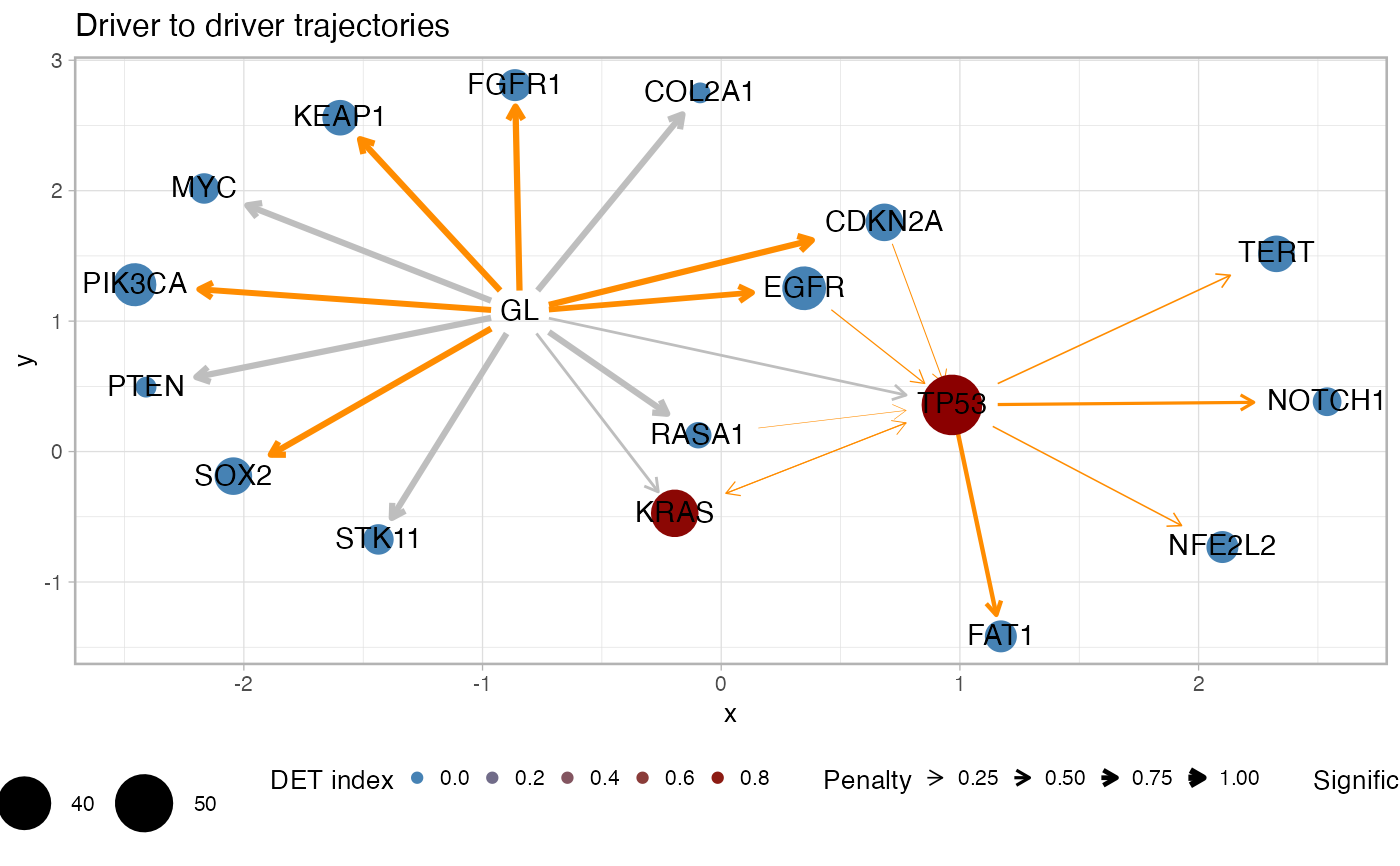
# Reduce the number of nodes cutting off low-frequencies one
plot_drivers_graph(TRACERx_NEJM_2017_REVOLVER, min.occurrences = 5)
#> 
#> =-=-=-=-=-=-=-=-=-=-=-=-=-=-=-=-=-=-
#>  Enrichment test for incoming edges
#> =-=-=-=-=-=-=-=-=-=-=-=-=-=-=-=-=-=-
#> # A tibble: 15 × 15
#>    estimate    p.value conf.low conf.high method alternative from  to    POS_POS
#>       <dbl>      <dbl>    <dbl>     <dbl> <chr>  <chr>       <chr> <chr>   <int>
#>  1   Inf       3.10e-8    11.5        Inf Fishe… greater     EGFR  TP53       13
#>  2   Inf       3.16e-7    15.0        Inf Fishe… greater     TP53  FAT1        7
#>  3   Inf       2.01e-6     8.13       Inf Fishe… greater     CDKN… TP53       10
#>  4   Inf       2.95e-6    11.9        Inf Fishe… greater     TP53  TERT        6
#>  5   Inf       7.88e-6     7.08       Inf Fishe… greater     KRAS  TP53        9
#>  6   Inf       2.67e-5     9.10       Inf Fishe… greater     TP53  NFE2…       5
#>  7   Inf       2.67e-5     9.10       Inf Fishe… greater     TP53  NOTC…       5
#>  8   Inf       9.14e-4     2.67       Inf Fishe… greater     GL    EGFR       20
#>  9   Inf       9.14e-4     2.67       Inf Fishe… greater     GL    PIK3…      20
#> 10   Inf       1.64e-3     3.21       Inf Fishe… greater     RASA1 TP53        5
#> 11   Inf       8.06e-3     1.75       Inf Fishe… greater     GL    CDKN…      14
#> 12   Inf       8.06e-3     1.75       Inf Fishe… greater     GL    SOX2       14
#> 13     3.26    1.52e-2     1.31       Inf Fishe… greater     TP53  KRAS        8
#> 14   Inf       1.64e-2     1.45       Inf Fishe… greater     GL    KEAP1      12
#> 15   Inf       4.69e-2     1.03       Inf Fishe… greater     GL    FGFR1       9
#> # ℹ 6 more variables: POS_NEG <int>, NEG_POS <int>, NEG_NEG <int>,
#> #   alpha_level <dbl>, N <int>, psign <lgl>
#> Warning: Removed 1 row containing missing values or values outside the scale range
#> (`geom_point()`).


# As above, but with a more stringent test
plot_drivers_graph(TRACERx_NEJM_2017_REVOLVER, min.occurrences = 5, alpha_level = 0.01)
#> 
#> =-=-=-=-=-=-=-=-=-=-=-=-=-=-=-=-=-=-
#>  Enrichment test for incoming edges
#> =-=-=-=-=-=-=-=-=-=-=-=-=-=-=-=-=-=-
#> # A tibble: 12 × 15
#>    estimate    p.value conf.low conf.high method alternative from  to    POS_POS
#>       <dbl>      <dbl>    <dbl>     <dbl> <chr>  <chr>       <chr> <chr>   <int>
#>  1      Inf    3.10e-8    11.5        Inf Fishe… greater     EGFR  TP53       13
#>  2      Inf    3.16e-7    15.0        Inf Fishe… greater     TP53  FAT1        7
#>  3      Inf    2.01e-6     8.13       Inf Fishe… greater     CDKN… TP53       10
#>  4      Inf    2.95e-6    11.9        Inf Fishe… greater     TP53  TERT        6
#>  5      Inf    7.88e-6     7.08       Inf Fishe… greater     KRAS  TP53        9
#>  6      Inf    2.67e-5     9.10       Inf Fishe… greater     TP53  NFE2…       5
#>  7      Inf    2.67e-5     9.10       Inf Fishe… greater     TP53  NOTC…       5
#>  8      Inf    9.14e-4     2.67       Inf Fishe… greater     GL    EGFR       20
#>  9      Inf    9.14e-4     2.67       Inf Fishe… greater     GL    PIK3…      20
#> 10      Inf    1.64e-3     3.21       Inf Fishe… greater     RASA1 TP53        5
#> 11      Inf    8.06e-3     1.75       Inf Fishe… greater     GL    CDKN…      14
#> 12      Inf    8.06e-3     1.75       Inf Fishe… greater     GL    SOX2       14
#> # ℹ 6 more variables: POS_NEG <int>, NEG_POS <int>, NEG_NEG <int>,
#> #   alpha_level <dbl>, N <int>, psign <lgl>
#> Warning: Removed 1 row containing missing values or values outside the scale range
#> (`geom_point()`).