2. Plotting data • CNAqc

library(CNAqc)
#> ✔ Loading CNAqc, 'Copy Number Alteration quality check'. Support : <https://caravagn.github.io/CNAqc/>
require(dplyr)
#> Loading required package: dplyr
#> 
#> Attaching package: 'dplyr'
#> The following objects are masked from 'package:stats':
#> 
#>     filter, lag
#> The following objects are masked from 'package:base':
#> 
#>     intersect, setdiff, setequal, union

All CNAqc plotting functions use:

ggplot for panel plots;
ggpubr and cowplot for multi-panel figures assembly.

# Dataset available with the package 
data('example_dataset_CNAqc', package = 'CNAqc')

x = CNAqc::init(
  mutations = example_dataset_CNAqc$mutations, 
  cna = example_dataset_CNAqc$cna,
  purity = example_dataset_CNAqc$purity,
  ref = 'hg19')
#> 
#> ── CNAqc - CNA Quality Check ───────────────────────────────────────────────────
#> ℹ Using reference genome coordinates for: hg19.
#> ✔ Found annotated driver mutations: TTN, CTCF, and TP53.
#> ✔ Fortified calls for 12963 somatic mutations: 12963 SNVs (100%) and 0 indels.
#> ! CNAs have no CCF, assuming clonal CNAs (CCF = 1).
#> ✔ Fortified CNAs for 267 segments: 267 clonal and 0 subclonal.
#> ✔ 12963 mutations mapped to clonal CNAs.

print(x)
#> ── [ CNAqc ] MySample 12963 mutations in 267 segments (267 clonal, 0 subclonal).
#> 
#> ── Clonal CNAs
#> 
#>    2:2  [n = 7478, L = 1483 Mb] ■■■■■■■■■■■■■■■■■■■■■■■■■■■  { CTCF }
#>    4:2  [n = 1893, L =  331 Mb] ■■■■■■■
#>    3:2  [n = 1625, L =  357 Mb] ■■■■■■
#>    2:1  [n = 1563, L =  420 Mb] ■■■■■■  { TTN }
#>    3:0  [n =  312, L =  137 Mb] ■
#>    2:0  [n =   81, L =   39 Mb]   { TP53 }
#>   16:2  [n =    4, L =    0 Mb] 
#>   25:2  [n =    2, L =    1 Mb] 
#>    3:1  [n =    2, L =    1 Mb] 
#>  106:1  [n =    1, L =    0 Mb]
#> ℹ Sample Purity: 89% ~ Ploidy: 4.
#> ℹ There are 3 annotated driver(s) mapped to clonal CNAs.
#>          chr      from        to ref alt  DP NV       VAF driver_label is_driver
#>         chr2 179431633 179431634   C   T 117 77 0.6581197          TTN      TRUE
#>        chr16  67646006  67646007   C   T 120 54 0.4500000         CTCF      TRUE
#>        chr17   7577106   7577107   G   C  84 78 0.9285714         TP53      TRUE

Plotting copy number segments

Segments plots

CNAqc can plot genome-wide segments showing major and minor allele counts as red and blue bars. Bottom circles annotate breakpoints; by default this plot has limited y-axis and breakpoints for segments outside the plot (e.g. very high amplifications) are in black. Areas in the genome that are mapped to the most prevalent karyotype are shadowed by default.

# Default plot
plot_segments(x)
#> Scale for fill is already present.
#> Adding another scale for fill, which will replace the existing scale.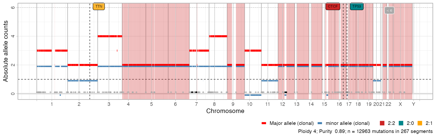

Note: the colour scheme in CNAqc is fixed for certain segments. The colour scheme is adopted also for other information, e.g., to report the segment where a certain driver is mapped.

An alternative circular layout plot is available.

# Circular layout
plot_segments(x, circular = TRUE)

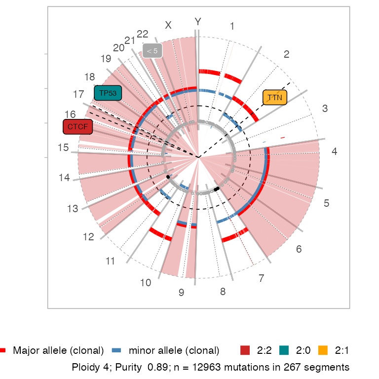
Customising segments plot

# Shadow other segments
plot_segments(x, highlight = c("2:1", "2:0", "2:2")) + 
  ggplot2::labs(title = "Annotate different karyotypes")
#> Scale for fill is already present.
#> Adding another scale for fill, which will replace the existing scale.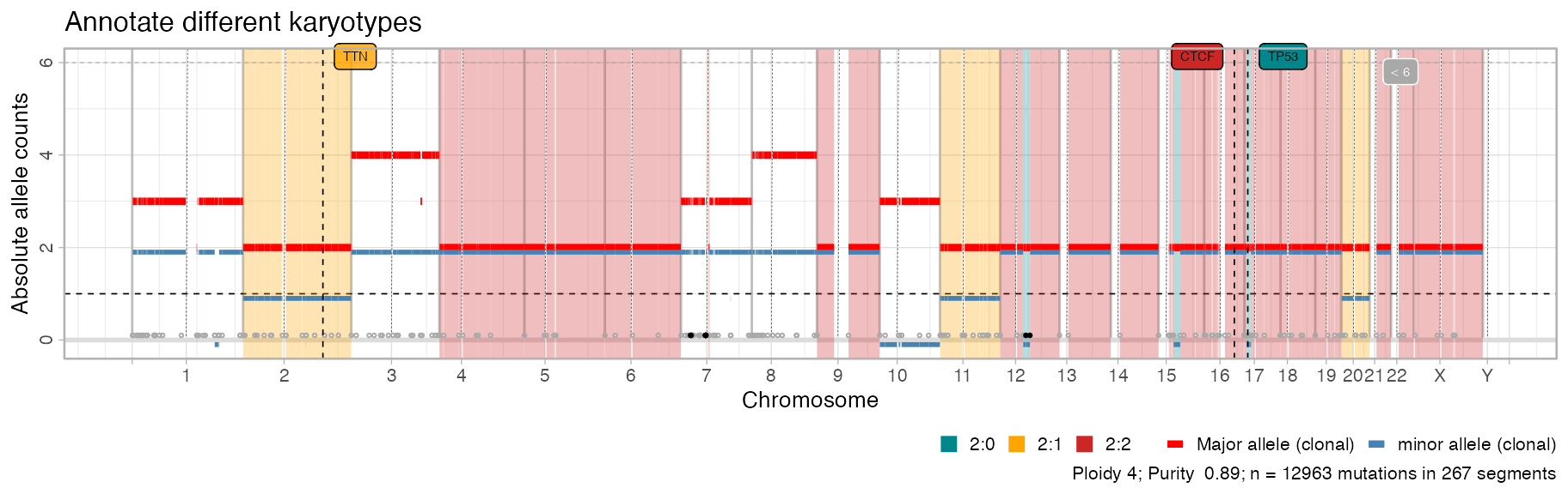


# Subset the genome
plot_segments(x, chromosomes = 'chr17') + ggplot2::labs(title = "Chromosome 17 zoom")
#> Scale for fill is already present.
#> Adding another scale for fill, which will replace the existing scale.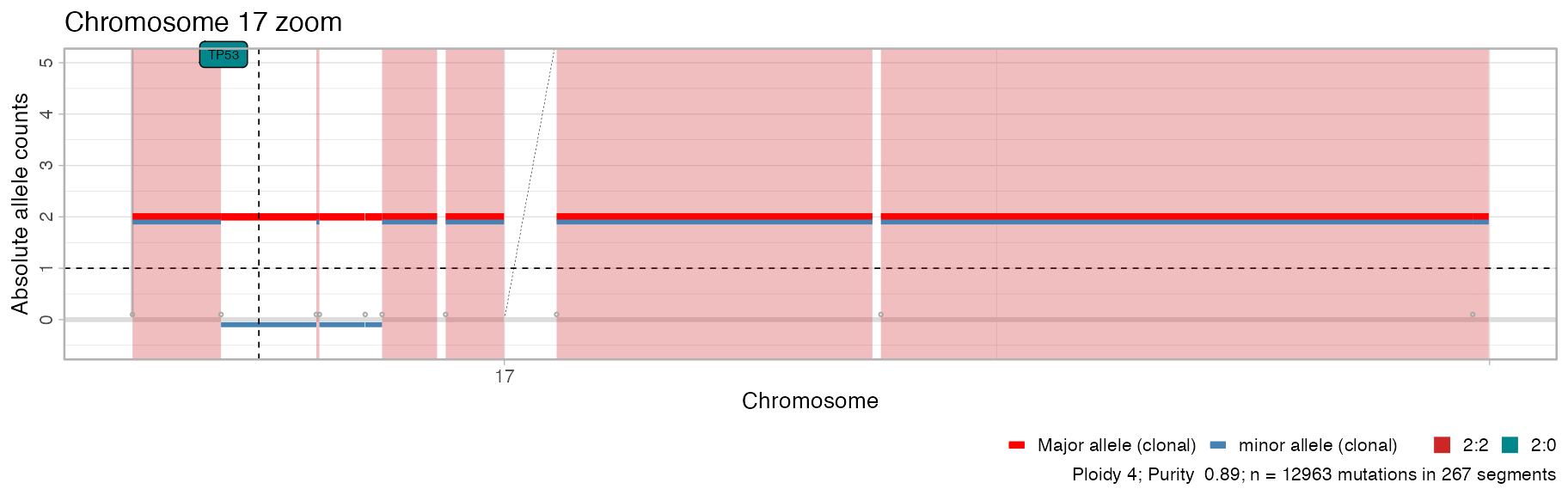

plot_segments(x, chromosomes = c('chr17', 'chr13')) + ggplot2::labs(title = "Chromosome 17 and 13 zoom")
#> Scale for fill is already present.
#> Adding another scale for fill, which will replace the existing scale.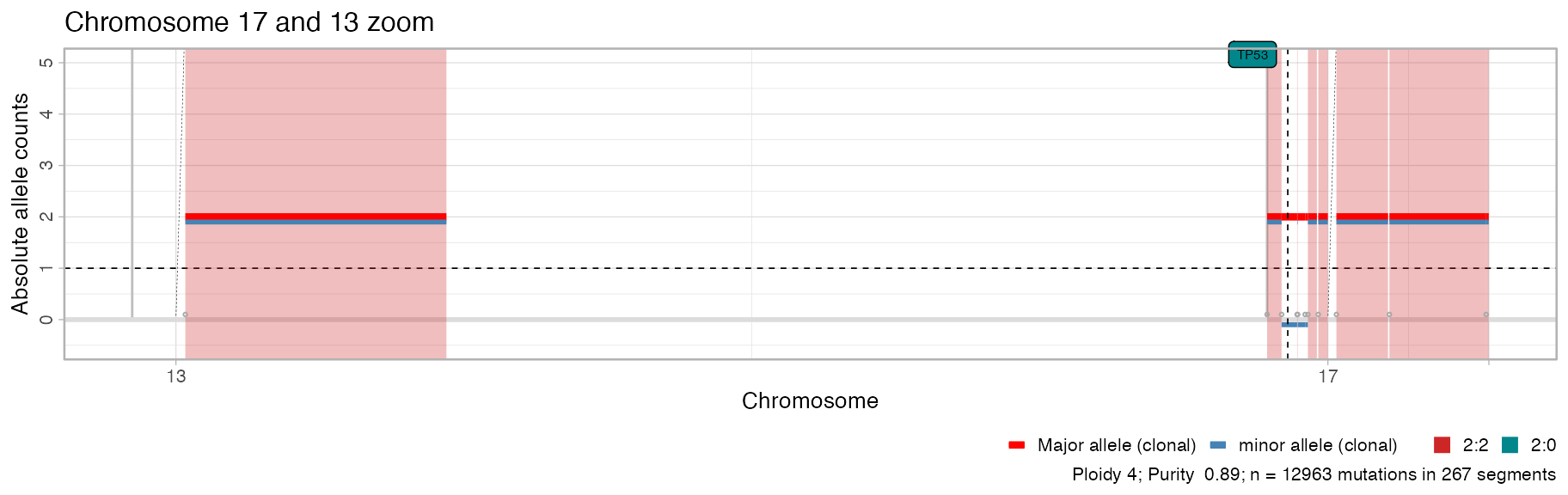


# Total copy number
plot_segments(x, cn = 'total') + ggplot2::labs(title = "Total copy number")
#> Scale for fill is already present.
#> Adding another scale for fill, which will replace the existing scale.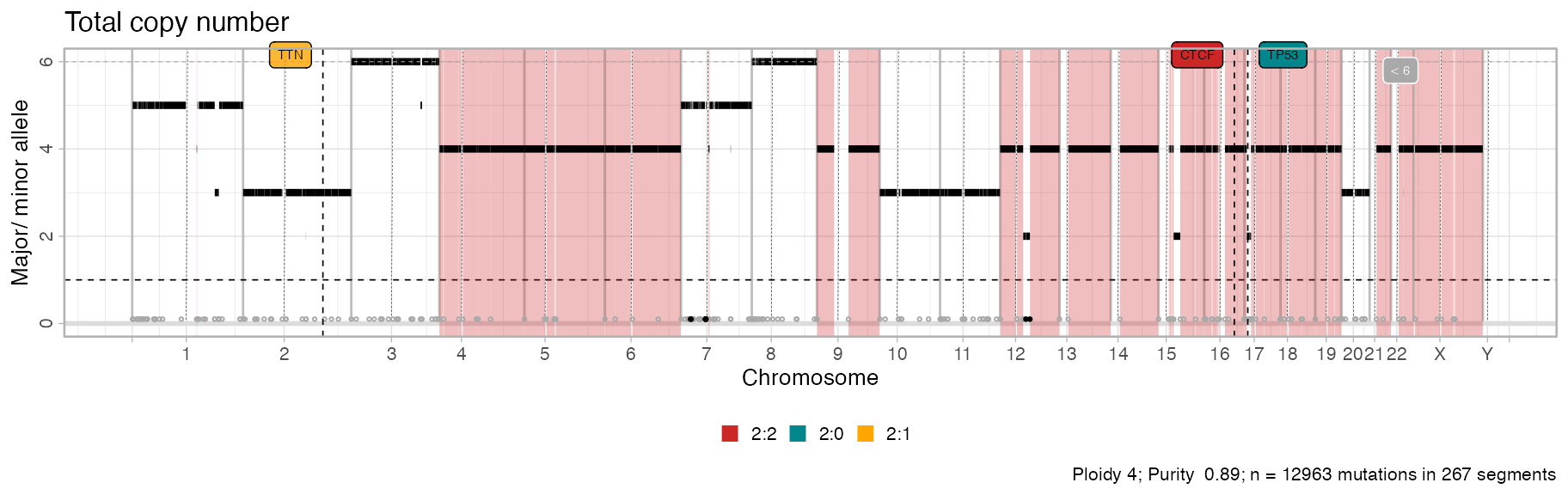

Subclonal CNAs

We use the PCAWG object released with the package

CNAqc::example_PCAWG %>% print()
#> ── [ CNAqc ]  293736 mutations in 667 segments (654 clonal, 13 subclonal). Genom
#> 
#> ── Clonal CNAs
#> 
#>   2:1  [n = 88422, L =   692 Mb] ■■■■■■■■■■■■■■■■■■■■■■■■■■■
#>   3:2  [n = 58384, L =   417 Mb] ■■■■■■■■■■■■■■■■■■  { BRAF }
#>   3:1  [n = 48704, L =   380 Mb] ■■■■■■■■■■■■■■■
#>   3:0  [n = 26622, L =   360 Mb] ■■■■■■■■  { CDKN2A }
#>   2:2  [n = 25290, L =   253 Mb] ■■■■■■■■
#>   3:3  [n = 16790, L =   115 Mb] ■■■■■
#>   2:0  [n =  5374, L =    67 Mb] ■■
#>   4:0  [n =  1752, L =    22 Mb] ■  { TP53 }
#>   4:2  [n =  1441, L =    11 Mb] 
#>   1:1  [n =   855, L =     9 Mb]
#> 
#> ── Subclonal CNAs (showing up to 10 segments)
#> 
#>  chr11@55700000  [n =  10468, L =  78.75 Mb]   2:1 (0.21)   2:2 (0.79) ■■■■■■■■■■
#>  chr11@17365005  [n =   5389, L =  31.55 Mb]   2:1 (0.21)   2:2 (0.79) ■■■■■
#>   chr11@5372292  [n =   1014, L =  11.99 Mb]   2:1 (0.21)   2:2 (0.79) 
#>    chr11@202253  [n =    610, L =   5.17 Mb]   2:1 (0.22)   2:2 (0.78) 
#>  chr11@48918601  [n =    542, L =   2.68 Mb]   2:1 (0.25)   2:2 (0.75) 
#>   chr6@82432583  [n =    301, L =   1.81 Mb]   2:1 (0.19)   2:2 (0.81) 
#>  chr11@51600000  [n =    290, L =    4.1 Mb]   2:1 (0.26)   2:2 (0.74) 
#>   chr6@81896364  [n =     69, L =   0.54 Mb]   2:1 (0.19)   2:2 (0.81) 
#>   chr6@93956180  [n =     41, L =   0.11 Mb]    2:1 (0.2)    2:2 (0.8) 
#>   chr8@42633277  [n =     13, L =   0.26 Mb]   2:1 (0.28)   2:2 (0.72)
#> ℹ Sample Purity: 73.4% ~ Ploidy: 3.
#> ℹ There are 3 annotated driver(s) mapped to clonal CNAs.
#>          chr      from        to ref alt DP NV       VAF driver_label is_driver
#>        chr17   7577082   7577082   C   T 78 70 0.8974359         TP53      TRUE
#>         chr7 140453136 140453136   A   T 95 54 0.5684211         BRAF      TRUE
#>         chr9  21971120  21971120   G   A 23 14 0.6086957       CDKN2A      TRUE
#> 
#> ──  PASS  Peaks QC closest: 199%, λ = 0.0059. Purity correction: 1%. ───────────
#> ℹ 2:1 ~ n = 88422 ( 74%) →  PASS  0.01     PASS  -0.006
#> ℹ 2:2 ~ n = 25290 ( 21%) →  PASS  0.01     PASS  0.002
#> ℹ 2:0 ~ n = 5374  (  4%) →  PASS  0.015    PASS  -0.001
#> ℹ 1:1 ~ n = 855   (0.7%) →  PASS  -0.006
#> ℹ 1:0 ~ n = 124   (0.1%) →  PASS  0.008
#> 
#> ── General peak QC (154430 mutations):  PASS  27  FAIL  13 - epsilon = 0.05. ───
#> ℹ 3:0 ~ n = 26622 ( 17%) →  PASS  3  FAIL  0
#> ℹ 3:1 ~ n = 48704 ( 32%) →  PASS  3  FAIL  0
#> ℹ 3:2 ~ n = 58384 ( 38%) →  PASS  3  FAIL  0
#> ℹ 3:3 ~ n = 16790 ( 11%) →  PASS  3  FAIL  0
#> ℹ 4:2 ~ n = 1441  (  1%) →  PASS  3  FAIL  1
#> ℹ 4:3 ~ n = 359   (  0%) →  PASS  3  FAIL  1
#> ℹ 5:3 ~ n = 132   (  0%) →  PASS  3  FAIL  2
#> ℹ 4:0 ~ n = 1752  (  1%) →  PASS  2  FAIL  2
#> ℹ 5:2 ~ n = 132   (  0%) →  PASS  2  FAIL  3
#> ℹ 6:3 ~ n = 114   (  0%) →  PASS  2  FAIL  4
#> 
#> ── Subclonal peaks QC (7 segments, initial state 2:1): linear 5 branching 0 eith
#> 
#> ──  PASS  Linear models
#> ℹ chr11@17365005 ~ (31.6Mb, n = 5389) 2:1 (21) + 2:2 (79) : A1B1 -> A1A2B1 -> A1A2B1B2 [100]
#> ℹ   chr11@202253 ~ (5.2Mb, n = 610) 2:1 (22) + 2:2 (78) : A1B1 -> A1A2B1 -> A1A2B1B2 [100]
#> ℹ chr11@51600000 ~ (4.1Mb, n = 290) 2:1 (26) + 2:2 (74) : A1B1 -> A1A2B1 -> A1A2B1B2 [75]
#> ℹ  chr11@5372292 ~ (12Mb, n = 1014) 2:1 (21) + 2:2 (79) : A1B1 -> A1A2B1 -> A1A2B1B2 [100]
#> ℹ chr11@55700000 ~ (78.8Mb, n = 10468) 2:1 (21) + 2:2 (79) : A1B1 -> A1A2B1 -> A1A2B1B2 [100]
#> 
#> ──  UNKNOWN  Either branching or linear models
#> ℹ chr11@48918601 ~ (2.7Mb, n = 542) 2:1 (25) + 2:2 (75) : A1B1 -> A1A2B1 -> A1A2B1B2 [100]; A1B1 -> A1A2B1 | A1A2B1B2 [100]; A1B1 -> A1A2B1B2 -> A2B1B2 [100]
#> ℹ  chr6@82432583 ~ (1.8Mb, n = 301) 2:1 (19) + 2:2 (81) : A1B1 -> A1A2B1 -> A1A2B1B2 [100]; A1B1 -> A1A2B1 | A1A2B1B2 [100]; A1B1 -> A1A2B1B2 -> A2B1B2 [100]
#> ✔ Cancer Cell Fraction (CCF) data available for karyotypes:1:0, 1:1, 2:0, 2:1, and 2:2.
#> ✔  PASS  CCF via ENTROPY.
#> ✔  PASS  CCF via ENTROPY.
#> ✔  PASS  CCF via ENTROPY.
#> ✔  PASS  CCF via ENTROPY.
#> ✔  PASS  CCF via ENTROPY.

Subclonal segments of each subclone have different colours compared to red/blue clonal segments.

plot_segments(CNAqc::example_PCAWG)
#> Scale for fill is already present.
#> Adding another scale for fill, which will replace the existing scale.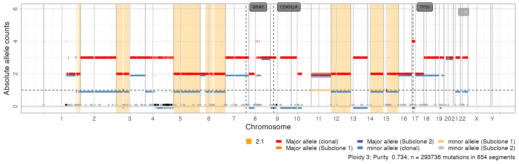

Note: the CCF of each subclone is not reported in this plot.

Segments summaries

Based on parameter type, function plot_karyotypes reports:

type = 'percentage', the proportion of genome covered by each segment (default);
type = 'number', the counts of segments per karyotype.

ggpubr::ggarrange(
  plot_karyotypes(x),
  plot_karyotypes(x, type = 'number'),
  common.legend = TRUE,
  legend = 'bottom'
)

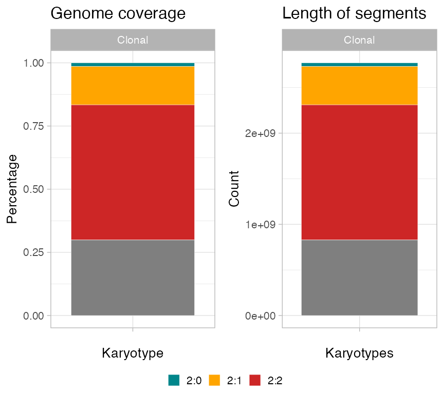
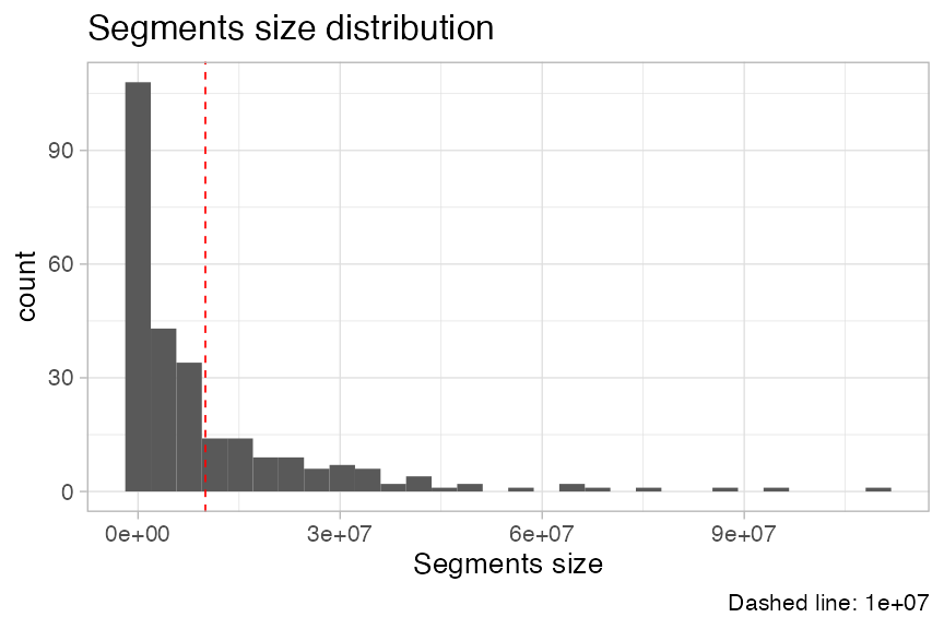
We can also plot the segments length distribution, which is used to detect fragmentation patterns.

plot_segment_size_distribution(x)

Plotting mutations

Data histograms

Read counts information can be plot using plot_data_histogram as histograms.

ggpubr::ggarrange(
  plot_data_histogram(x, which = 'VAF'),
  plot_data_histogram(x, which = 'DP'),
  plot_data_histogram(x, which = 'NV'),
  ncol = 3,
  nrow = 1
  )
#> Warning: Removed 8 rows containing missing values (`geom_bar()`).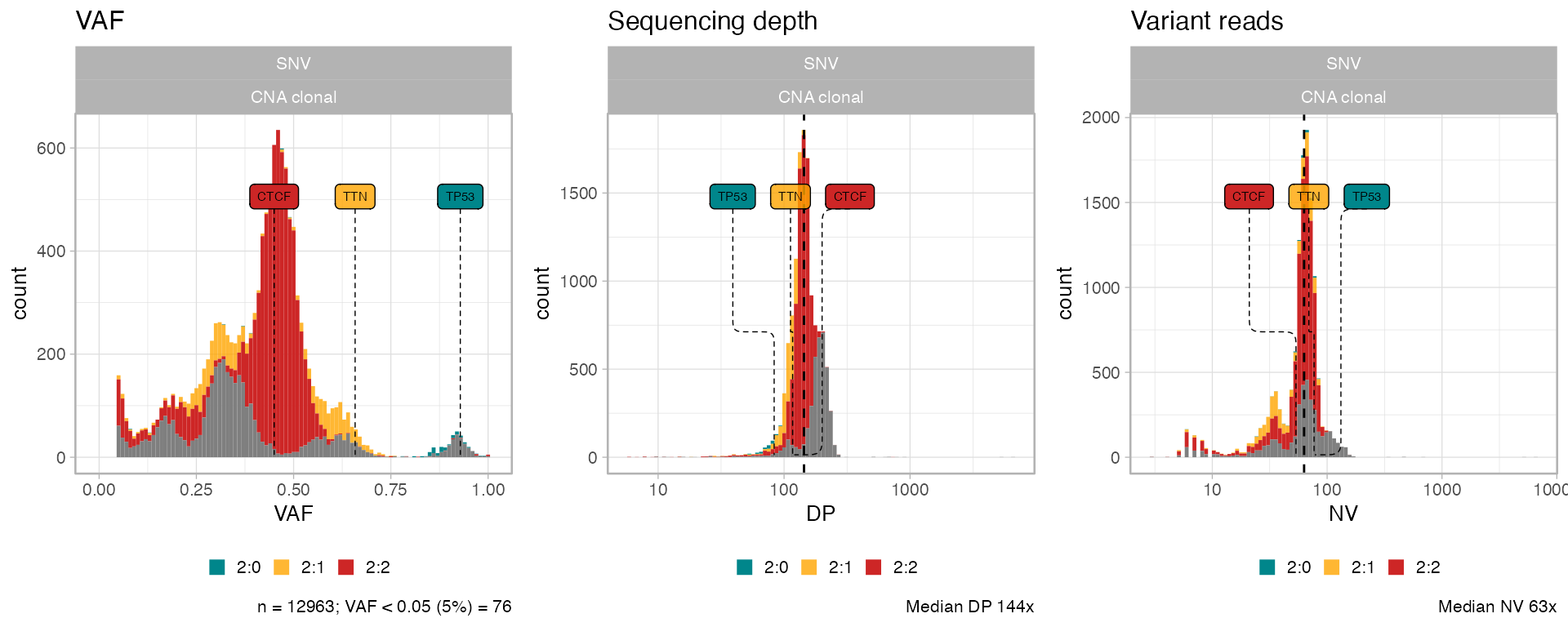

Note: if you compute CCFs you can use plot_data_histogram(x, which = 'CCF') as well.

Segment-specific VAFs

VAFs per segment, split by chromosome, can help identify miscalled segments (i.e., for segments with the same major/minor allele copies the VAF distributions should be similar)

inspect_segment(x)
#> Warning: The `<scale>` argument of `guides()` cannot be `FALSE`. Use "none" instead as
#> of ggplot2 3.3.4.
#> ℹ The deprecated feature was likely used in the CNAqc package.
#>   Please report the issue at <https://github.com/caravagnalab/CNAqc/issues>.
#> This warning is displayed once every 8 hours.
#> Call `lifecycle::last_lifecycle_warnings()` to see where this warning was
#> generated.
#> Warning: Removed 30 rows containing missing values (`geom_bar()`).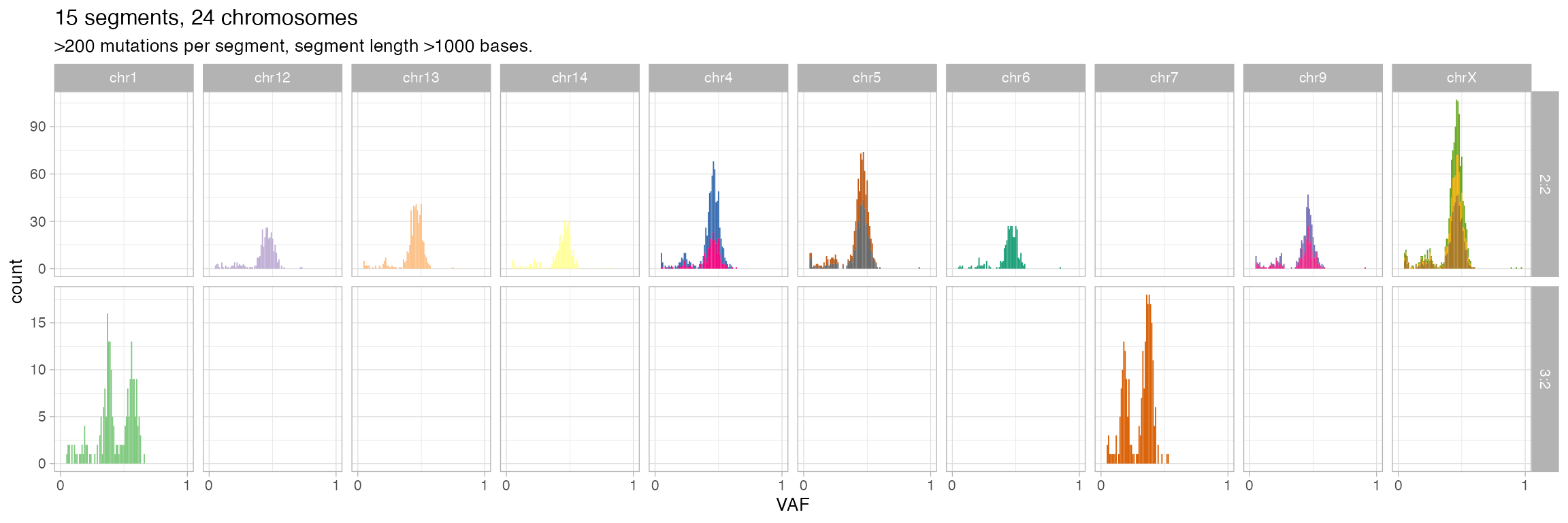

# With facet from a data histogram
plot_data_histogram(x, which = 'VAF') + 
  ggplot2::facet_grid(karyotype~chr, scales = 'free')
#> Warning: Removed 56 rows containing missing values (`geom_bar()`).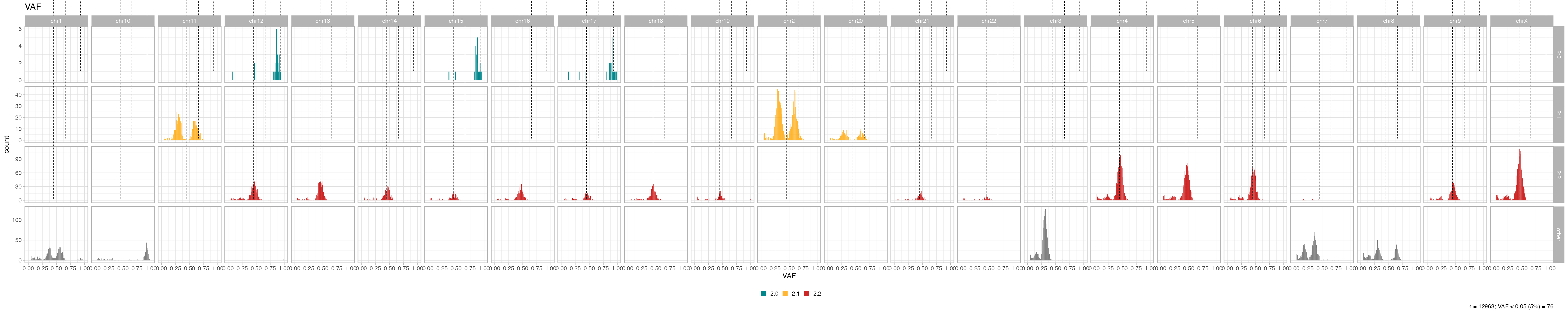

Genome-wide mutation data

Genome-wide plots that follow the layout of plot_segments are avaiable to view the genome-wide distributions of the number of mutations, their VAF and depth. VAF and depth-plotting functions (scatterplots) can subset the input data to speed up rendering and reduce the size of output files - by default \(5000\) points are shown Counts plot, instead, bin the genome locations by one megabase (\(10^6\) bases).

# All genome, all data - counts of mutations per megabase
plot_gw_counts(x)
#> Warning: The dot-dot notation (`..count..`) was deprecated in ggplot2 3.4.0.
#> ℹ Please use `after_stat(count)` instead.
#> ℹ The deprecated feature was likely used in the CNAqc package.
#>   Please report the issue at <https://github.com/caravagnalab/CNAqc/issues>.
#> This warning is displayed once every 8 hours.
#> Call `lifecycle::last_lifecycle_warnings()` to see where this warning was
#> generated.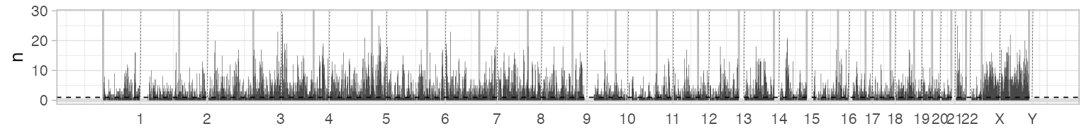

# An example effect of downsampling the data
ggpubr::ggarrange(
  plot_gw_depth(x, N = 1000),
  plot_gw_depth(x),
  plot_gw_depth(x, N = 10000),
  ncol = 1
)
#> Warning: Removed 24 rows containing missing values (`geom_segment()`).
#> Warning: Removed 24 rows containing missing values (`geom_rect()`).
#> Warning: Removed 1 rows containing missing values (`geom_hline()`).
#> Removed 1 rows containing missing values (`geom_hline()`).
#> Warning: Removed 24 rows containing missing values (`geom_segment()`).
#> Warning: Removed 24 rows containing missing values (`geom_rect()`).
#> Warning: Removed 1 rows containing missing values (`geom_hline()`).
#> Removed 1 rows containing missing values (`geom_hline()`).
#> Warning: Removed 24 rows containing missing values (`geom_segment()`).
#> Warning: Removed 24 rows containing missing values (`geom_rect()`).
#> Warning: Removed 1 rows containing missing values (`geom_hline()`).
#> Removed 1 rows containing missing values (`geom_hline()`).

Combined plots

The default S3 plot function layouts a panel with segments in bottom, and all other genome-wide plots on top. This function aligns plots on the vertical axis, and stretch their relative height to obtain a nice layout.

# The actual plot function
cowplot::plot_grid(
  plot_gw_counts(x),
  plot_gw_vaf(x, N = 10000),
  plot_gw_depth(x, N = 10000),
  plot_segments(x),
  align = 'v',
  nrow = 4,
  rel_heights = c(.15, .15, .15, .8))
#> Scale for fill is already present.
#> Adding another scale for fill, which will replace the existing scale.
#> Warning: Removed 24 rows containing missing values (`geom_segment()`).
#> Warning: Removed 24 rows containing missing values (`geom_rect()`).
#> Warning: Removed 1 rows containing missing values (`geom_hline()`).
#> Removed 1 rows containing missing values (`geom_hline()`).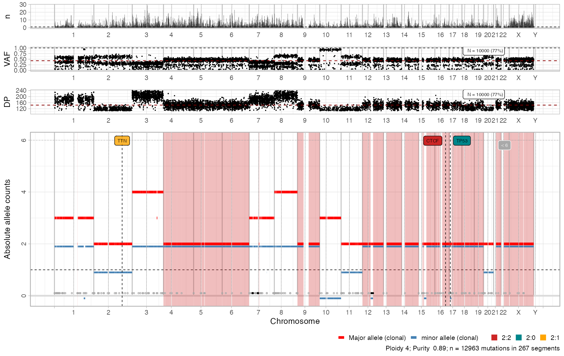

Cohort plots

One can have multiple CNAqc objects - i.e., work with a cohort of objects - when working with

a group of distinct patients;
multiple samples from the same patient;
multiple calls from the same sample;

Assuming all input objects have the same reference, cohort cohort-level plots are possible.

# Object 1
x = CNAqc::init(
  mutations = example_dataset_CNAqc$mutations, 
  cna = example_dataset_CNAqc$cna,
  purity = example_dataset_CNAqc$purity,
  ref = 'hg19'
  )
#> 
#> ── CNAqc - CNA Quality Check ───────────────────────────────────────────────────
#> ℹ Using reference genome coordinates for: hg19.
#> ✔ Found annotated driver mutations: TTN, CTCF, and TP53.
#> ✔ Fortified calls for 12963 somatic mutations: 12963 SNVs (100%) and 0 indels.
#> ! CNAs have no CCF, assuming clonal CNAs (CCF = 1).
#> ✔ Fortified CNAs for 267 segments: 267 clonal and 0 subclonal.
#> ✔ 12963 mutations mapped to clonal CNAs.

# Object 1 with some modifications
y = CNAqc::init(
  mutations = example_dataset_CNAqc$mutations, 
  cna = example_dataset_CNAqc$cna %>%
    mutate(
      Major = ifelse(chr %in% c("chr3", "chr4", "chr1"), 1, Major),
      minor = ifelse(chr %in% c("chr3", "chr4", "chr1"), 1, minor)
      ),
  purity = example_dataset_CNAqc$purity,
  ref = 'hg19')
#> 
#> ── CNAqc - CNA Quality Check ───────────────────────────────────────────────────
#> ℹ Using reference genome coordinates for: hg19.
#> ✔ Found annotated driver mutations: TTN, CTCF, and TP53.
#> ✔ Fortified calls for 12963 somatic mutations: 12963 SNVs (100%) and 0 indels.
#> ! CNAs have no CCF, assuming clonal CNAs (CCF = 1).
#> ✔ Fortified CNAs for 267 segments: 267 clonal and 0 subclonal.
#> ✔ 12963 mutations mapped to clonal CNAs.

# PCAWG sample
z = CNAqc::example_PCAWG

# Inputs need to be wrapped in a named list
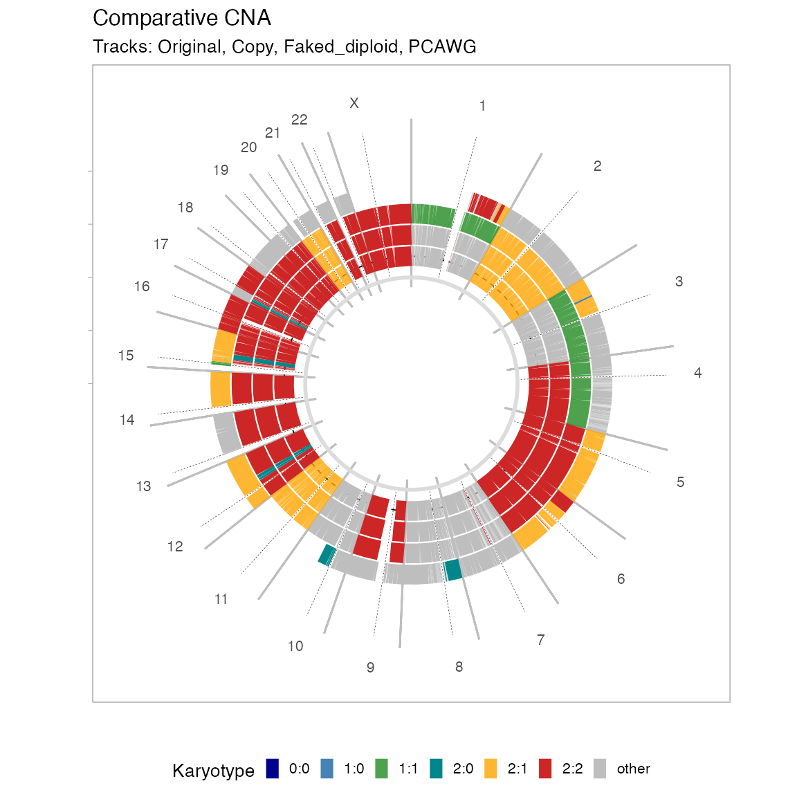
inputs = list(`Original` = x, `Copy` = x, `Faked_diploid` = y, `PCAWG` = z)

Copy number segments

The frequency of deletions and amplifications relative to diploid are shown by using a certain binning (step \(\delta\)) of the tumour genome. Here by deletion we define anything with 0 copies of the minor allele, and by amplification anything with \(\geq 3\) total copies (sum of the minor and major alleles).

# Comparative CNA plot - default delta
plot_multisample_CNA(inputs)
#> 
#> ── Breaking input segments at 100 Kb resolution
#> Warning: replacing previous import 'cli::num_ansi_colors' by
#> 'crayon::num_ansi_colors' when loading 'easypar'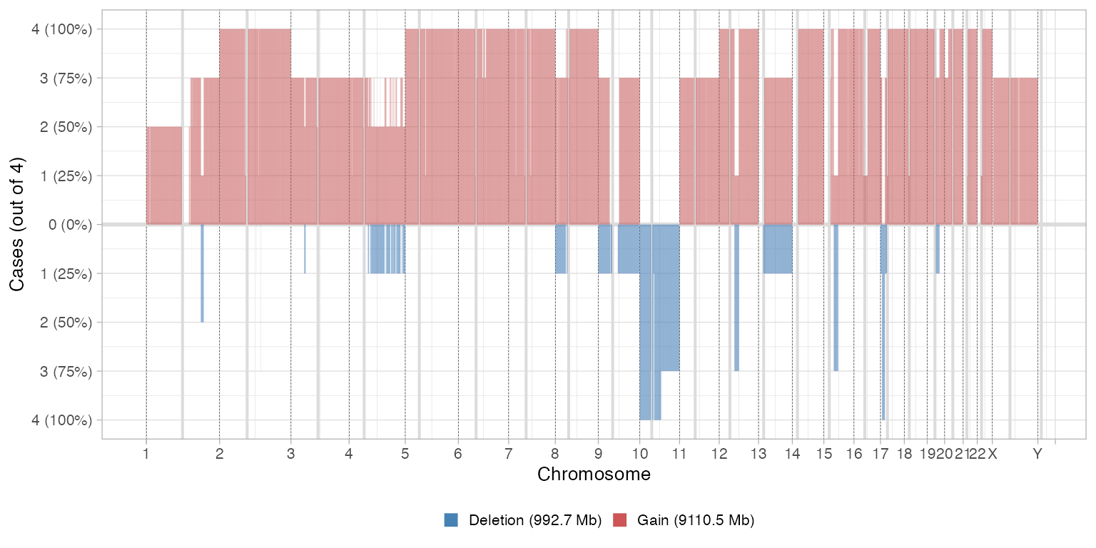

The binning \(\delta\) of the tumour genome can be changed to get larger/ shorter segments

# Comparative CNA plot - 10 Mb delta
plot_multisample_CNA(inputs, delta = 1e7)
#> 
#> ── Breaking input segments at 10000 Kb resolution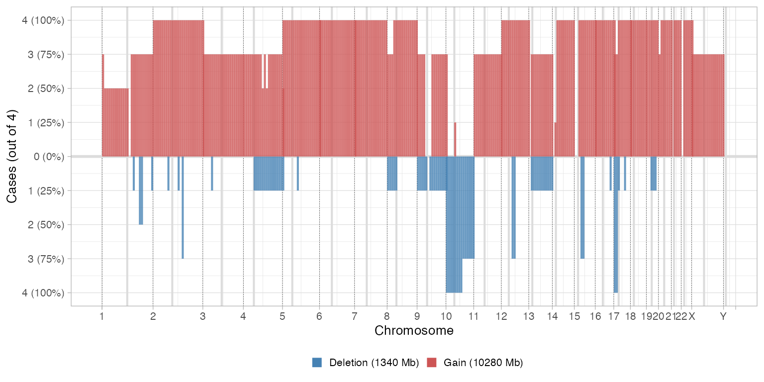

A circular layout is also possible, with no binning or transformation of the data.

# Comparative CNA plot
plot_multisample_CNA(inputs, layout = 'circular')