library(CNAqc)
#> ✔ Loading CNAqc, 'Copy Number Alteration quality check'. Support : <https://caravagn.github.io/CNAqc/>

# Extra packages
require(dplyr)
#> Loading required package: dplyr
#>
#> Attaching package: 'dplyr'
#> The following objects are masked from 'package:stats':
#>
#>     filter, lag
#> The following objects are masked from 'package:base':
#>
#>     intersect, setdiff, setequal, union
require(vcfR)
#> Loading required package: vcfR
#>
#>    *****       ***   vcfR   ***       *****
#>    This is vcfR 1.15.0
#>      browseVignettes('vcfR') # Documentation
#>      citation('vcfR') # Citation
#>    *****       *****      *****       *****
We work with MSeq data discussed in the main preprint for
CNAqc, replicating one analysis for patient
Set06.
The data we used is hosted at the GitHub repository caravagnalab/CNAqc_datasets.
Mutation data
We download from Github a VCF file for MSeq sample
Set06, and load it using the vcfR package.
VCF_url = "https://raw.githubusercontent.com/caravagnalab/CNAqc_datasets/main/MSeq_Set06/Mutations/Set.06.WGS.merged_filtered.vcf"

# Download, load and cancel data
download.file(VCF_url, "Set.06.WGS.merged_filtered.vcf",)

set6 = vcfR::read.vcfR("Set.06.WGS.merged_filtered.vcf")
#> Scanning file to determine attributes.
#> File attributes:
#>   meta lines: 47
#>   header_line: 48
#>   variant count: 43053
#>   column count: 16
#> Meta line 47 read in.
#> All meta lines processed.
#> gt matrix initialized.
#> Character matrix gt created.
#>   Character matrix gt rows: 43053
#>   Character matrix gt cols: 16
#>   skip: 0
#>   nrows: 43053
#>   row_num: 0
#> Processed variant 1000Processed variant 2000Processed variant 3000Processed variant 4000Processed variant 5000Processed variant 6000Processed variant 7000Processed variant 8000Processed variant 9000Processed variant 10000Processed variant 11000Processed variant 12000Processed variant 13000Processed variant 14000Processed variant 15000Processed variant 16000Processed variant 17000Processed variant 18000Processed variant 19000Processed variant 20000Processed variant 21000Processed variant 22000Processed variant 23000Processed variant 24000Processed variant 25000Processed variant 26000Processed variant 27000Processed variant 28000Processed variant 29000Processed variant 30000Processed variant 31000Processed variant 32000Processed variant 33000Processed variant 34000Processed variant 35000Processed variant 36000Processed variant 37000Processed variant 38000Processed variant 39000Processed variant 40000Processed variant 41000Processed variant 42000Processed variant 43000Processed variant: 43053
#> All variants processed

file.remove("Set.06.WGS.merged_filtered.vcf")
#> [1] TRUE

# VCF
print(set6)
#> ***** Object of Class vcfR *****
#> 7 samples
#> 24 CHROMs
#> 43,053 variants
#> Object size: 43.5 Mb
#> 0 percent missing data
#> *****        *****         *****
We extract all the information we need, using the tidy data representation format.
# INFO fields
info_tidy = vcfR::extract_info_tidy(set6)

# Fixed fields (genomic coordinates)
fix_tidy = set6@fix %>%
  as_tibble %>%
  rename(
    chr = CHROM,
    from = POS,
    ref = REF,
    alt = ALT
  ) %>%
  mutate(from = as.numeric(from), to = from + nchar(alt))

# Genotypes
geno_tidy = vcfR::extract_gt_tidy(set6) %>%
  group_split(Indiv)
#> Extracting gt element GT
#> Extracting gt element GQ
#> Extracting gt element GOF
#> Extracting gt element NR
#> Extracting gt element GL
#> Extracting gt element NV

# Sample mutations in the CNAqc format
sample_mutations = lapply(geno_tidy, function(x) {
  bind_cols(info_tidy, fix_tidy) %>%
    full_join(x, by = "Key") %>%
    mutate(DP = as.numeric(gt_NR), NV = as.numeric(gt_NV)) %>%
    mutate(VAF = NV / DP) %>%
    dplyr::select(chr, from, to, ref, alt, NV, DP, VAF, everything()) %>%
    filter(!is.na(VAF), VAF > 0)
})

# A list for all samples available
names(sample_mutations) = sapply(sample_mutations, function(x) x$Indiv[1])
sample_mutations = sample_mutations[!is.na(names(sample_mutations))]
We have all the somatic mutations called for Set06.
print(sample_mutations)
#> $Set6_42
#> # A tibble: 33,245 × 46
#>    chr     from     to ref      alt      NV    DP    VAF   Key FR     MMLQ   TCR
#>    <chr>  <dbl>  <dbl> <chr>    <chr> <dbl> <dbl>  <dbl> <int> <chr> <dbl> <int>
#>  1 chr1   30923  30924 G        T         2    41 0.0488     1 0.42…    37    98
#>  2 chr1   83906  83907 A        G         1    56 0.0179     2 0.28…    37   132
#>  3 chr1   83911  83930 AAGAGAG… TAGA…     2    59 0.0339     3 0.07…    37   133
#>  4 chr1   83933  83934 A        G         1    59 0.0169     4 0.00…   100   141
#>  5 chr1  137123 137124 T        G         5    44 0.114      5 0.14…    37    87
#>  6 chr1  797474 797475 G        T         6    75 0.08       6 0.12…    37   222
#>  7 chr1  809123 809124 G        A         2    92 0.0217     7 0.14…    37   235
#>  8 chr1  809135 809136 C        T         2    91 0.0220     8 0.14…    37   236
#>  9 chr1  812625 812642 GCTGTGG… TCTG…     1    90 0.0111     9 0.14…    37   223
#> 10 chr1  815277 815278 T        C        10    70 0.143     10 0.35…    37   196
#> # ℹ 33,235 more rows
#> # ℹ 34 more variables: HP <int>, WE <int>, Source <chr>, FS <chr>, WS <int>,
#> #   PP <chr>, TR <chr>, NF <chr>, TCF <int>, NR <chr>, TC <int>, END <chr>,
#> #   MGOF <chr>, SbPval <chr>, START <chr>, ReadPosRankSum <chr>, MQ <chr>,
#> #   QD <dbl>, SC <chr>, BRF <dbl>, HapScore <chr>, Size <chr>, ID <chr>,
#> #   QUAL <chr>, FILTER <chr>, INFO <chr>, Indiv <chr>, gt_GT <chr>,
#> #   gt_GQ <chr>, gt_GOF <chr>, gt_NR <chr>, gt_GL <chr>, gt_NV <chr>, …
#>
#> $Set6_44
#> # A tibble: 32,960 × 46
#>    chr     from     to ref   alt      NV    DP    VAF   Key FR      MMLQ   TCR
#>    <chr>  <dbl>  <dbl> <chr> <chr> <dbl> <dbl>  <dbl> <int> <chr>  <dbl> <int>
#>  1 chr1   30923  30924 G     T         2    20 0.1        1 0.4275    37    98
#>  2 chr1   83906  83907 A     G         3    39 0.0769     2 0.2857    37   132
#>  3 chr1   83933  83934 A     G         3    46 0.0652     4 0.0000   100   141
#>  4 chr1  137123 137124 T     G         1    29 0.0345     5 0.1438    37    87
#>  5 chr1  797474 797475 G     T         5    78 0.0641     6 0.1291    37   222
#>  6 chr1  809123 809124 G     A         3    67 0.0448     7 0.1429    37   235
#>  7 chr1  809135 809136 C     T         2    66 0.0303     8 0.1429    37   236
#>  8 chr1  815277 815278 T     C         4    70 0.0571    10 0.3569    37   196
#>  9 chr1  815316 815319 GTT   ATC       3    80 0.0375    11 0.1403    37   191
#> 10 chr1  819221 819225 GTTA  ATTC      2    55 0.0364    12 0.0715    23   198
#> # ℹ 32,950 more rows
#> # ℹ 34 more variables: HP <int>, WE <int>, Source <chr>, FS <chr>, WS <int>,
#> #   PP <chr>, TR <chr>, NF <chr>, TCF <int>, NR <chr>, TC <int>, END <chr>,
#> #   MGOF <chr>, SbPval <chr>, START <chr>, ReadPosRankSum <chr>, MQ <chr>,
#> #   QD <dbl>, SC <chr>, BRF <dbl>, HapScore <chr>, Size <chr>, ID <chr>,
#> #   QUAL <chr>, FILTER <chr>, INFO <chr>, Indiv <chr>, gt_GT <chr>,
#> #   gt_GQ <chr>, gt_GOF <chr>, gt_NR <chr>, gt_GL <chr>, gt_NV <chr>, …
#>
#> $Set6_45
#> # A tibble: 32,782 × 46
#>    chr     from     to ref      alt      NV    DP    VAF   Key FR     MMLQ   TCR
#>    <chr>  <dbl>  <dbl> <chr>    <chr> <dbl> <dbl>  <dbl> <int> <chr> <dbl> <int>
#>  1 chr1   30923  30924 G        T         2    42 0.0476     1 0.42…    37    98
#>  2 chr1   83906  83907 A        G         3    57 0.0526     2 0.28…    37   132
#>  3 chr1   83911  83930 AAGAGAG… TAGA…     5    57 0.0877     3 0.07…    37   133
#>  4 chr1   83933  83934 A        G         3    59 0.0508     4 0.00…   100   141
#>  5 chr1  137123 137124 T        G         3    34 0.0882     5 0.14…    37    87
#>  6 chr1  797474 797475 G        T         3    64 0.0469     6 0.12…    37   222
#>  7 chr1  809123 809124 G        A         3    71 0.0423     7 0.14…    37   235
#>  8 chr1  809135 809136 C        T         3    75 0.04       8 0.14…    37   236
#>  9 chr1  815277 815278 T        C         9    81 0.111     10 0.35…    37   196
#> 10 chr1  815316 815319 GTT      ATC       3    89 0.0337    11 0.14…    37   191
#> # ℹ 32,772 more rows
#> # ℹ 34 more variables: HP <int>, WE <int>, Source <chr>, FS <chr>, WS <int>,
#> #   PP <chr>, TR <chr>, NF <chr>, TCF <int>, NR <chr>, TC <int>, END <chr>,
#> #   MGOF <chr>, SbPval <chr>, START <chr>, ReadPosRankSum <chr>, MQ <chr>,
#> #   QD <dbl>, SC <chr>, BRF <dbl>, HapScore <chr>, Size <chr>, ID <chr>,
#> #   QUAL <chr>, FILTER <chr>, INFO <chr>, Indiv <chr>, gt_GT <chr>,
#> #   gt_GQ <chr>, gt_GOF <chr>, gt_NR <chr>, gt_GL <chr>, gt_NV <chr>, …
#>
#> $Set6_46
#> # A tibble: 33,907 × 46
#>    chr     from     to ref      alt      NV    DP    VAF   Key FR     MMLQ   TCR
#>    <chr>  <dbl>  <dbl> <chr>    <chr> <dbl> <dbl>  <dbl> <int> <chr> <dbl> <int>
#>  1 chr1   30923  30924 G        T         2    22 0.0909     1 0.42…    37    98
#>  2 chr1   83906  83907 A        G         3    35 0.0857     2 0.28…    37   132
#>  3 chr1   83933  83934 A        G         6    38 0.158      4 0.00…   100   141
#>  4 chr1  137123 137124 T        G         1    30 0.0333     5 0.14…    37    87
#>  5 chr1  797474 797475 G        T         4    65 0.0615     6 0.12…    37   222
#>  6 chr1  809123 809124 G        A         6    96 0.0625     7 0.14…    37   235
#>  7 chr1  809135 809136 C        T         5    94 0.0532     8 0.14…    37   236
#>  8 chr1  812625 812642 GCTGTGG… TCTG…     3    87 0.0345     9 0.14…    37   223
#>  9 chr1  815277 815278 T        C        10    69 0.145     10 0.35…    37   196
#> 10 chr1  815316 815319 GTT      ATC       3    85 0.0353    11 0.14…    37   191
#> # ℹ 33,897 more rows
#> # ℹ 34 more variables: HP <int>, WE <int>, Source <chr>, FS <chr>, WS <int>,
#> #   PP <chr>, TR <chr>, NF <chr>, TCF <int>, NR <chr>, TC <int>, END <chr>,
#> #   MGOF <chr>, SbPval <chr>, START <chr>, ReadPosRankSum <chr>, MQ <chr>,
#> #   QD <dbl>, SC <chr>, BRF <dbl>, HapScore <chr>, Size <chr>, ID <chr>,
#> #   QUAL <chr>, FILTER <chr>, INFO <chr>, Indiv <chr>, gt_GT <chr>,
#> #   gt_GQ <chr>, gt_GOF <chr>, gt_NR <chr>, gt_GL <chr>, gt_NV <chr>, …
#>
#> $Set6_47
#> # A tibble: 32,814 × 46
#>    chr     from     to ref      alt      NV    DP    VAF   Key FR     MMLQ   TCR
#>    <chr>  <dbl>  <dbl> <chr>    <chr> <dbl> <dbl>  <dbl> <int> <chr> <dbl> <int>
#>  1 chr1   30923  30924 G        T         3    12 0.25       1 0.42…    37    98
#>  2 chr1   83906  83907 A        G         6    41 0.146      2 0.28…    37   132
#>  3 chr1   83933  83934 A        G         7    39 0.179      4 0.00…   100   141
#>  4 chr1  137123 137124 T        G         7    38 0.184      5 0.14…    37    87
#>  5 chr1  797474 797475 G        T         4    68 0.0588     6 0.12…    37   222
#>  6 chr1  809123 809124 G        A         4    84 0.0476     7 0.14…    37   235
#>  7 chr1  809135 809136 C        T         2    84 0.0238     8 0.14…    37   236
#>  8 chr1  812625 812642 GCTGTGG… TCTG…     4    71 0.0563     9 0.14…    37   223
#>  9 chr1  815277 815278 T        C         6    67 0.0896    10 0.35…    37   196
#> 10 chr1  815316 815319 GTT      ATC       2    68 0.0294    11 0.14…    37   191
#> # ℹ 32,804 more rows
#> # ℹ 34 more variables: HP <int>, WE <int>, Source <chr>, FS <chr>, WS <int>,
#> #   PP <chr>, TR <chr>, NF <chr>, TCF <int>, NR <chr>, TC <int>, END <chr>,
#> #   MGOF <chr>, SbPval <chr>, START <chr>, ReadPosRankSum <chr>, MQ <chr>,
#> #   QD <dbl>, SC <chr>, BRF <dbl>, HapScore <chr>, Size <chr>, ID <chr>,
#> #   QUAL <chr>, FILTER <chr>, INFO <chr>, Indiv <chr>, gt_GT <chr>,
#> #   gt_GQ <chr>, gt_GOF <chr>, gt_NR <chr>, gt_GL <chr>, gt_NV <chr>, …
#>
#> $Set6_48
#> # A tibble: 32,859 × 46
#>    chr     from     to ref      alt      NV    DP    VAF   Key FR     MMLQ   TCR
#>    <chr>  <dbl>  <dbl> <chr>    <chr> <dbl> <dbl>  <dbl> <int> <chr> <dbl> <int>
#>  1 chr1   30923  30924 G        T         3    14 0.214      1 0.42…    37    98
#>  2 chr1   83906  83907 A        G         2    28 0.0714     2 0.28…    37   132
#>  3 chr1   83933  83934 A        G         3    36 0.0833     4 0.00…   100   141
#>  4 chr1  137123 137124 T        G         2    36 0.0556     5 0.14…    37    87
#>  5 chr1  797474 797475 G        T         6    69 0.0870     6 0.12…    37   222
#>  6 chr1  809123 809124 G        A         5    76 0.0658     7 0.14…    37   235
#>  7 chr1  809135 809136 C        T         5    78 0.0641     8 0.14…    37   236
#>  8 chr1  812625 812642 GCTGTGG… TCTG…     1    62 0.0161     9 0.14…    37   223
#>  9 chr1  815277 815278 T        C         6    58 0.103     10 0.35…    37   196
#> 10 chr1  815316 815319 GTT      ATC       4    71 0.0563    11 0.14…    37   191
#> # ℹ 32,849 more rows
#> # ℹ 34 more variables: HP <int>, WE <int>, Source <chr>, FS <chr>, WS <int>,
#> #   PP <chr>, TR <chr>, NF <chr>, TCF <int>, NR <chr>, TC <int>, END <chr>,
#> #   MGOF <chr>, SbPval <chr>, START <chr>, ReadPosRankSum <chr>, MQ <chr>,
#> #   QD <dbl>, SC <chr>, BRF <dbl>, HapScore <chr>, Size <chr>, ID <chr>,
#> #   QUAL <chr>, FILTER <chr>, INFO <chr>, Indiv <chr>, gt_GT <chr>,
#> #   gt_GQ <chr>, gt_GOF <chr>, gt_NR <chr>, gt_GL <chr>, gt_NV <chr>, …
Copy Number data
Sequenza calls are available in the same repository.
We use an extra function to load a solution (so we can easily compare multiple runs etc etc.).
# Load Sequenza output
load_SQ_output = function(URL, sample, run)
{
  # We can directly read them from remote URLs
  segments_file = paste0(URL, run, '/', sample, '.smoothedSegs.txt')
  purity_file = paste0(URL, run, '/', sample, '_confints_CP.txt')

  # Get segments
  segments = readr::read_tsv(segments_file, col_types = readr::cols()) %>%
    dplyr::rename(
      chr = chromosome,
      from = start.pos,
      to = end.pos,
      Major = A,
      minor = B
    ) %>%
    dplyr::select(chr, from, to, Major, minor, dplyr::everything())

  # Get purity and ploidy
  solutions = readr::read_tsv(purity_file, col_types = readr::cols())

  purity = solutions$cellularity[2]
  ploidy = solutions$ploidy.estimate[2]

  return(
    list(
      segments = segments,
      purity = purity,
      ploidy = ploidy
    )
  )
}
We can load the calls for 2 solutions of sample Set6_42;
we begin with our final, good solution.
Sequenza_URL = "https://raw.githubusercontent.com/caravagnalab/CNAqc_datasets/main/MSeq_Set06/Copy%20Number/"

# Final sequenza run (good calls)
Sequenza_good_calls = load_SQ_output(Sequenza_URL, sample = 'Set6_42', run = 'final')

print(Sequenza_good_calls)
#> $segments
#> # A tibble: 54 × 7
#>    chr        from        to Major minor   CNt      size
#>    <chr>     <dbl>     <dbl> <dbl> <dbl> <dbl>     <dbl>
#>  1 chr1    2847119  27674851     1     0     1  24827732
#>  2 chr1   27681534 120332727     1     1     2  92651193
#>  3 chr1  120333201 121485435     2     0     2   1152234
#>  4 chr1  142535470 246750621     1     1     2 104215151
#>  5 chr2    2500000  90500000     1     1     2  88000000
#>  6 chr2   96800000 240699373     1     1     2 143899373
#>  7 chr3    2500000  87900000     1     1     2  85400000
#>  8 chr3   93900000 195522430     1     1     2 101622430
#>  9 chr4    2500000  48200000     1     1     2  45700000
#> 10 chr4   52700000 188654276     1     1     2 135954276
#> # ℹ 44 more rows
#>
#> $purity
#> [1] 0.69
#>
#> $ploidy
#> [1] 2
Calls analysis
For this example we work with mutations found in sample
Set6_42.
# Single-nucleotide variants with VAF >5%
snvs = sample_mutations[['Set6_42']] %>%
    filter(ref %in% c('A', 'C', "T", 'G'), alt %in% c('A', 'C', "T", 'G')) %>%
    filter(VAF > 0.05)

# CNA segments and purity
cna = Sequenza_good_calls$segments
purity = Sequenza_good_calls$purity
Full CNAqc analysis. First we create the object.
# CNAqc data object
x = CNAqc::init(
  mutations = snvs,
  cna = cna,
  purity = purity,
  ref = "GRCh38")
#>
#> ── CNAqc - CNA Quality Check ───────────────────────────────────────────────────
#> ℹ Using reference genome coordinates for: GRCh38.
#> ✔ Fortified calls for 18858 somatic mutations: 18858 SNVs (100%) and 0 indels.
#> ! CNAs have no CCF, assuming clonal CNAs (CCF = 1).
#> ! Added segments length (in basepairs) to CNA segments.
#> ✔ Fortified CNAs for 54 segments: 54 clonal and 0 subclonal.
#> ✔ 17283 mutations mapped to clonal CNAs.

print(x)
#> ── [ CNAqc ] MySample 17283 mutations in 54 segments (54 clonal, 0 subclonal). G
#>
#> ── Clonal CNAs
#>
#>  1:1  [n = 14488, L =  2398 Mb] ■■■■■■■■■■■■■■■■■■■■■■■■■■■
#>  2:0  [n =  1552, L =   200 Mb] ■■■
#>  1:0  [n =   898, L =   141 Mb] ■■
#>  2:1  [n =   345, L =    43 Mb] ■
#> ℹ Sample Purity: 69% ~ Ploidy: 2.
Data
Show the CNA data for this sample.
cowplot::plot_grid(
  plot_gw_counts(x),
  plot_gw_vaf(x, N = 10000),
  plot_gw_depth(x, N = 10000),
  plot_segments(x, highlight = c("1:0", "1:1", "2:0", "2:1", '2:2')),
  align = 'v',
  nrow = 4,
  rel_heights = c(.15, .15, .15, .8))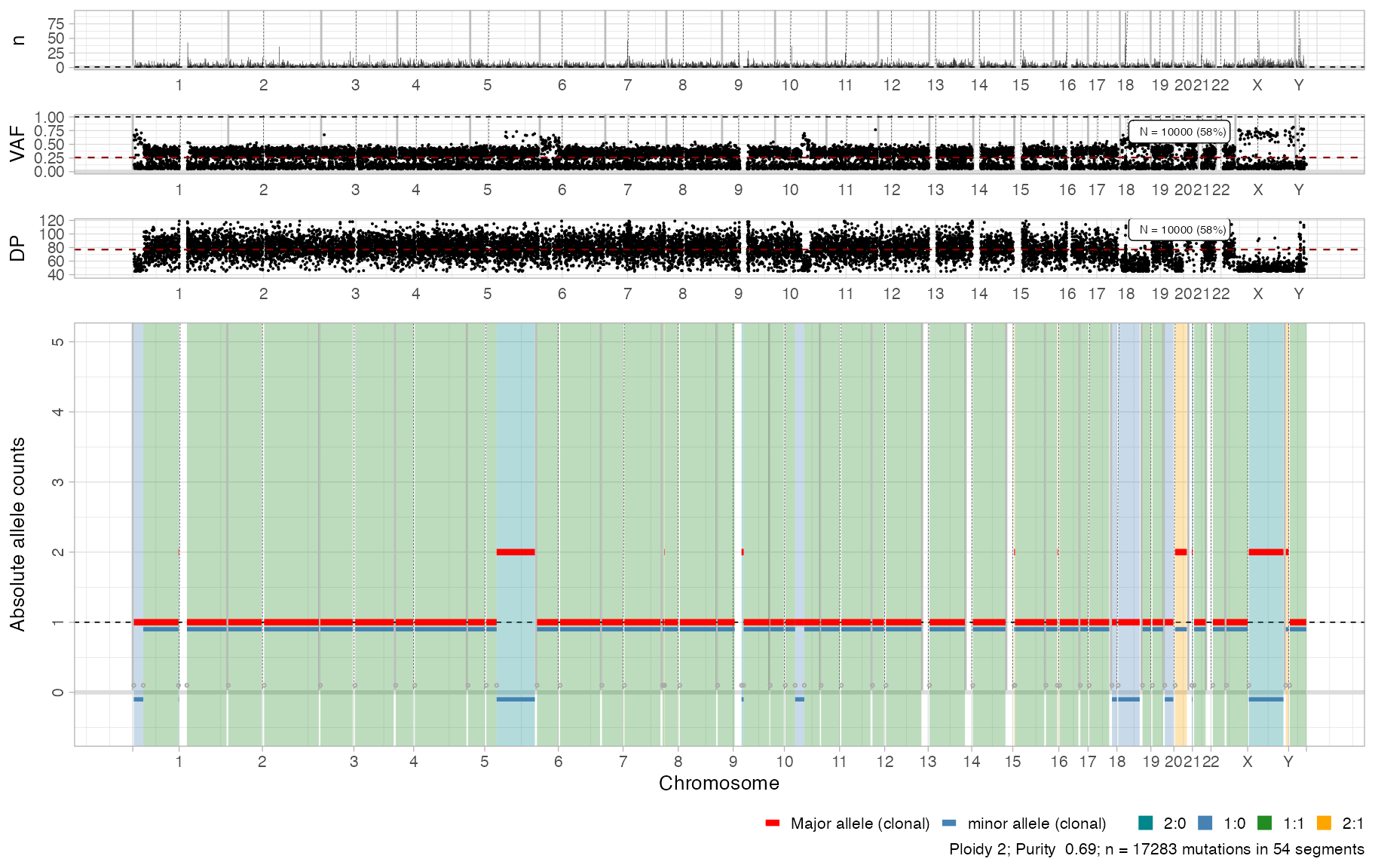
Show the mutation data for this sample.
ggpubr::ggarrange(
  plot_data_histogram(x, which = 'VAF'),
  plot_data_histogram(x, which = 'DP'),
  plot_data_histogram(x, which = 'NV'),
  ncol = 3,
  nrow = 1
  )
#> Warning: Removed 8 rows containing missing values or values outside the scale range
#> (`geom_bar()`).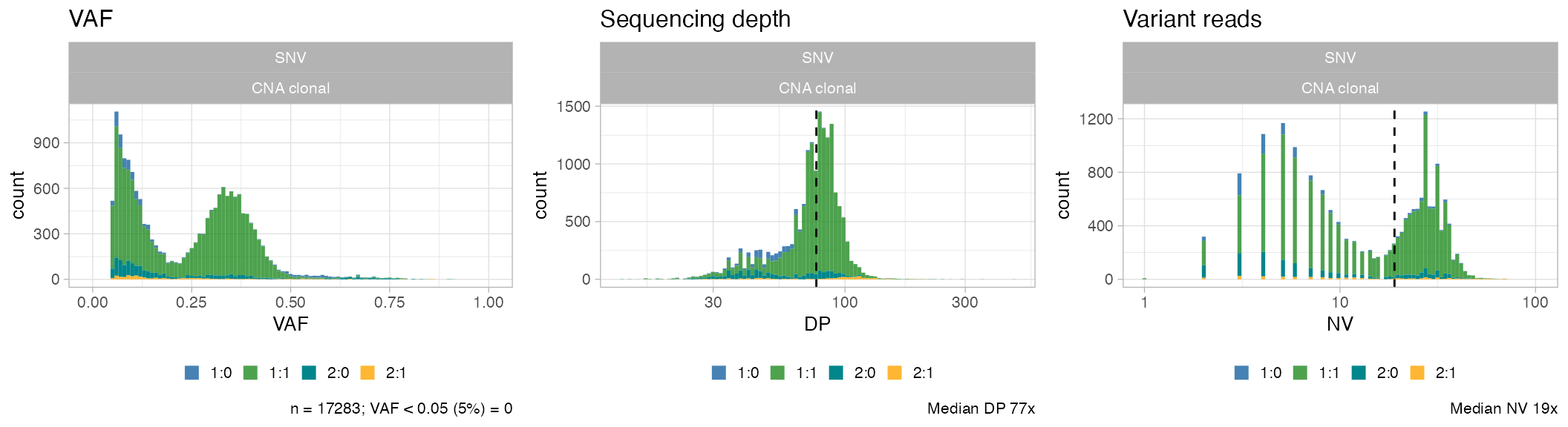
Peak detection
Perform peak detection and show its results.
# Peaks
x = CNAqc::analyze_peaks(x, matching_strategy = 'closest')
#>
#> ── Peak analysis: simple CNAs ──────────────────────────────────────────────────
#> ℹ Analysing 17283 mutations mapping to karyotype(s) 1:0, 1:1, 2:0, and 2:1.
#> ℹ Mixed type peak detection for karyotype 1:0 (898 mutations)
#> Warning: replacing previous import 'cli::num_ansi_colors' by
#> 'crayon::num_ansi_colors' when loading 'BMix'
#> Warning: replacing previous import 'crayon::%+%' by 'ggplot2::%+%' when loading
#> 'BMix'
#> ✔ Loading BMix, 'Binomial and Beta-Binomial univariate mixtures'. Support : <https://caravagnalab.github.io/BMix/>
#> Warning: replacing previous import 'cli::num_ansi_colors' by
#> 'crayon::num_ansi_colors' when loading 'easypar'
#> ℹ Mixed type peak detection for karyotype 1:1 (14488 mutations)
#> ℹ Mixed type peak detection for karyotype 2:0 (1552 mutations)
#> ℹ Mixed type peak detection for karyotype 2:1 (345 mutations)
#> # A tibble: 6 × 16
#> # Rowwise:
#>   mutation_multiplicity karyotype  peak delta_vaf     x     y counts_per_bin
#>                   <dbl> <chr>     <dbl>     <dbl> <dbl> <dbl>          <int>
#> 1                     1 1:0       0.527    0.0583 0.54  1.26              13
#> 2                     1 1:1       0.345    0.025  0.347 3.66             604
#> 3                     1 2:0       0.345    0.025  0.343 1.42              19
#> 4                     2 2:0       0.69     0.05   0.678 0.532              8
#> 5                     1 2:1       0.257    0.0138 0.288 1.47               7
#> 6                     2 2:1       0.513    0.0276 0.527 0.619              5
#> # ℹ 9 more variables: discarded <lgl>, from <chr>, offset_VAF <dbl>,
#> #   offset <dbl>, weight <dbl>, epsilon <dbl>, VAF_tolerance <dbl>,
#> #   matched <lgl>, QC <chr>
#> ✔ Peak detection PASS with r = -0.00516811972673077 - maximum purity error ε = 0.05.
#> Joining with `by = join_by(Major, minor)`
#> Joining with `by = join_by(karyotype)`
#>
#> ── Peak analysis: complex CNAs
#> ─────────────────────────────────────────────────
#> ℹ No karyotypes with >100 mutation(s).
#>
#> ── Peak analysis: subclonal CNAs ───────────────────────────────────────────────
#> ℹ No subclonal CNAs in this sample.

print(x)
#> ── [ CNAqc ] MySample 17283 mutations in 54 segments (54 clonal, 0 subclonal). G
#>
#> ── Clonal CNAs
#>
#>  1:1  [n = 14488, L =  2398 Mb] ■■■■■■■■■■■■■■■■■■■■■■■■■■■
#>  2:0  [n =  1552, L =   200 Mb] ■■■
#>  1:0  [n =   898, L =   141 Mb] ■■
#>  2:1  [n =   345, L =    43 Mb] ■
#> ℹ Sample Purity: 69% ~ Ploidy: 2.
#>
#> ──  PASS  Peaks QC closest: 107%, λ = -0.0052. Purity correction: -1%. ─────────
#> ℹ 1:0 ~ n = 898   (  5%) →  PASS  -0.011
#> ℹ 1:1 ~ n = 14488 ( 84%) →  PASS  -0.004
#> ℹ 2:0 ~ n = 1552  (  9%) →  PASS  0.004    PASS  0.012
#> ℹ 2:1 ~ n = 345   (  2%) →  FAIL  -0.123   FAIL  -0.026
For this sample these calls are passed by CNAqc.
# Do not assemble plots, and remove karyotypes with no data associated
plot_peaks_analysis(x, empty_plot = FALSE, assembly_plot = FALSE)
#> [[1]]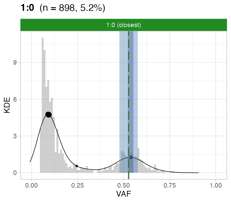
#>
#> [[2]]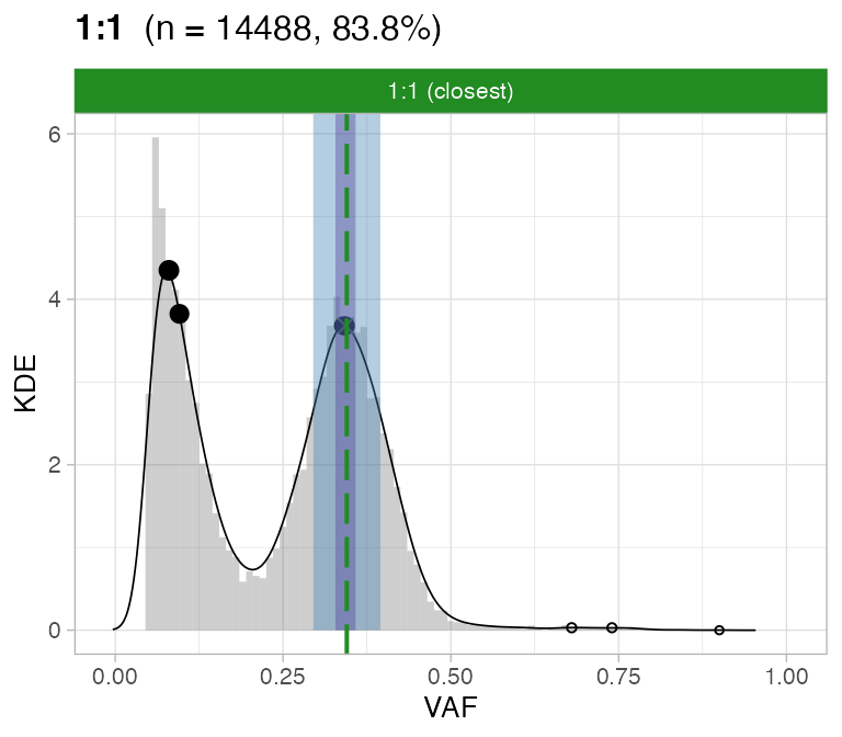
#>
#> [[3]]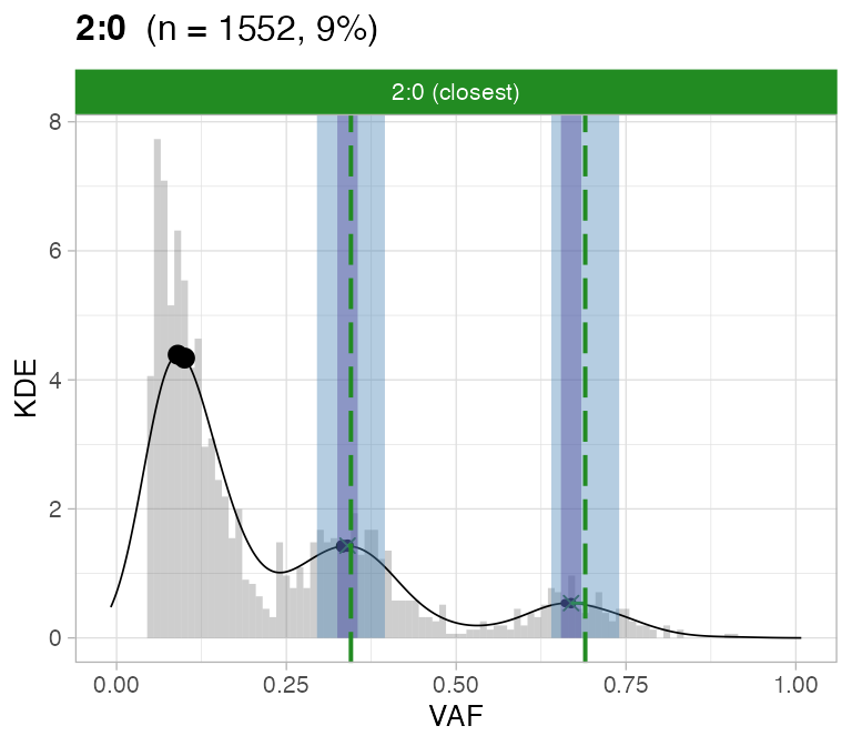
#>
#> [[4]]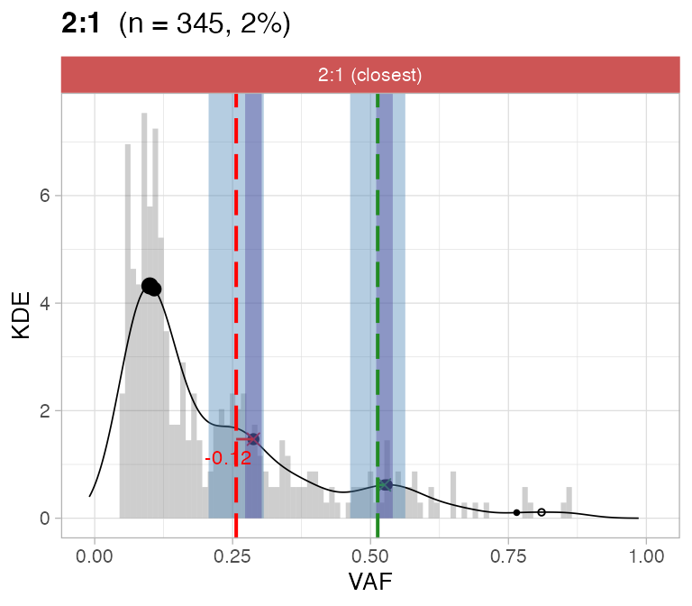
CCF
Perform CCF computation detection with the ENTROPY
method.
# CCF
x = CNAqc::compute_CCF(x, method = 'ENTROPY')
#> ── Computing mutation multiplicity for single-copy karyotype 1:0 ───────────────
#> ── Computing mutation multiplicity for single-copy karyotype 1:1 ───────────────
#> ── Computing mutation multiplicity for karyotype 2:0 using the entropy method. ─
#> ℹ Expected Binomial peak(s) for these calls (1 and 2 copies): 0.345 and 0.69
#> ℹ Mixing pre/ post aneuploidy: 0.74 and 0.26
#> ℹ Not assignamble area: [0.452830188679245; 0.622641509433962]
#> ── Computing mutation multiplicity for karyotype 2:1 using the entropy method. ─
#> ℹ Expected Binomial peak(s) for these calls (1 and 2 copies): 0.256505576208178 and 0.513011152416357
#> ℹ Mixing pre/ post aneuploidy: 0.7 and 0.3
#> ℹ Not assignamble area: [0.336842105263158; 0.442105263157895]

print(x)
#> ── [ CNAqc ] MySample 17283 mutations in 54 segments (54 clonal, 0 subclonal). G
#>
#> ── Clonal CNAs
#>
#>  1:1  [n = 14488, L =  2398 Mb] ■■■■■■■■■■■■■■■■■■■■■■■■■■■
#>  2:0  [n =  1552, L =   200 Mb] ■■■
#>  1:0  [n =   898, L =   141 Mb] ■■
#>  2:1  [n =   345, L =    43 Mb] ■
#> ℹ Sample Purity: 69% ~ Ploidy: 2.
#>
#> ──  PASS  Peaks QC closest: 107%, λ = -0.0052. Purity correction: -1%. ─────────
#> ℹ 1:0 ~ n = 898   (  5%) →  PASS  -0.011
#> ℹ 1:1 ~ n = 14488 ( 84%) →  PASS  -0.004
#> ℹ 2:0 ~ n = 1552  (  9%) →  PASS  0.004    PASS  0.012
#> ℹ 2:1 ~ n = 345   (  2%) →  FAIL  -0.123   FAIL  -0.026
#> ✔ Cancer Cell Fraction (CCF) data available for karyotypes:1:0, 1:1, 2:0, and 2:1.
#> ✔  PASS  CCF via ENTROPY.
#> ✔  PASS  CCF via ENTROPY.
#> ✔  PASS  CCF via ENTROPY.
#> ✔  PASS  CCF via ENTROPY.
CCF can be estimated well for this sample.
# Do not assemble plots, and remove karyotypes with no data associated
plot_CCF(x, assembly_plot = FALSE, empty_plot = FALSE)
#> [[1]]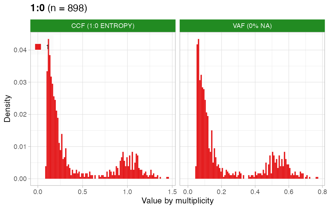
#>
#> [[2]]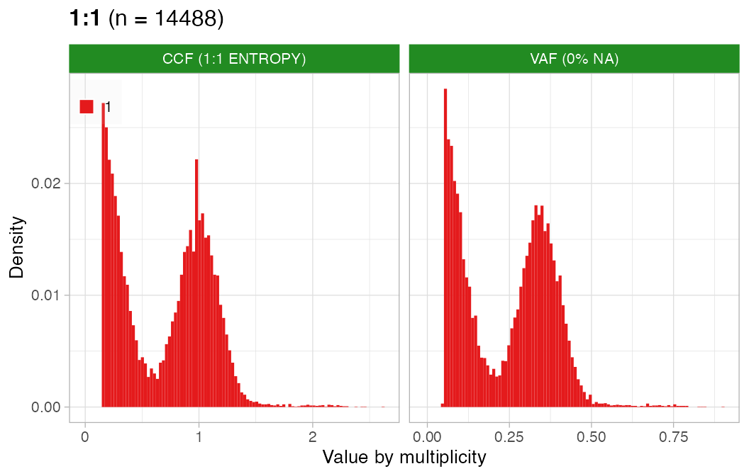
#>
#> [[3]]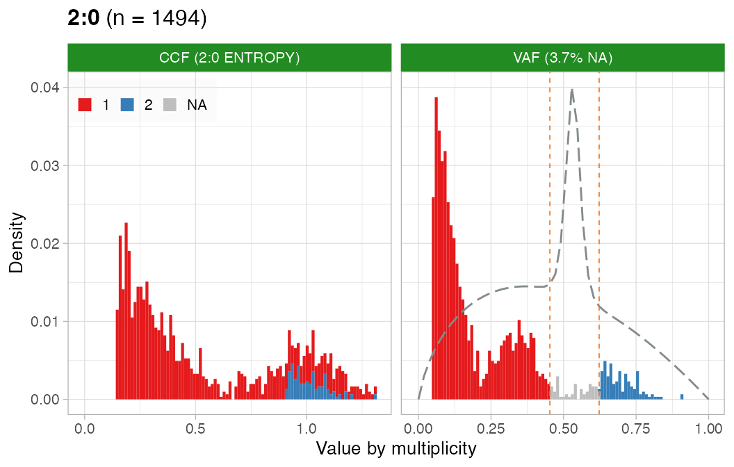
#>
#> [[4]]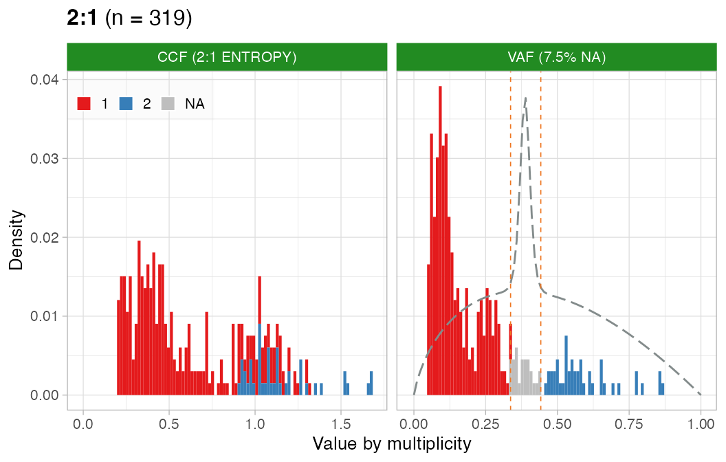
Other analyses
Smooth segments with gaps up to 10 megabases (does not affect segments in this sample).
x = CNAqc::smooth_segments(x)
#> → chr1 4 -4 @
#> → chr2 2 -2 @
#> → chr3 2 -2 @
#> → chr4 2 -2 @
#> → chr5 3 -3 @
#> → chr6 2 -2 @
#> → chr7 2 -2 @
#> → chr8 4 -4 @
#> → chr9 3 -3 @
#> → chr10 4 -4 @
#> → chr11 2 -2 @
#> → chr12 2 -2 @
#> → chr15 2 -2 @
#> → chr16 3 -3 @
#> → chr17 2 -2 @
#> → chr18 2 -2 @
#> → chr19 2 -2 @
#> → chr20 2 -2 @
#> → chr21 2 -2 @
#> → chrX 2 -2 @
#> → chrY 2 -2 @
#> ✔ Smoothed from 54 to 54 segments with 1e+06 gap (bases).
#> ℹ Creating a new CNAqc object. The old object will be retained in the $before_smoothing field.
#>
#> ── CNAqc - CNA Quality Check ───────────────────────────────────────────────────
#> ℹ Using reference genome coordinates for: GRCh38.
#> ✔ Fortified calls for 17283 somatic mutations: 17283 SNVs (100%) and 0 indels.
#> ✔ Fortified CNAs for 54 segments: 54 clonal and 0 subclonal.
#> Warning in map_mutations_to_clonal_segments(mutations, cna_clonal): [CNAqc] a
#> karyotype column is present in CNA calls, and will be overwritten
#> ✔ 17283 mutations mapped to clonal CNAs.

print(x)
#> ── [ CNAqc ] MySample 17283 mutations in 54 segments (54 clonal, 0 subclonal). G
#>
#> ── Clonal CNAs
#>
#>  1:1  [n = 14488, L =  2398 Mb] ■■■■■■■■■■■■■■■■■■■■■■■■■■■
#>  2:0  [n =  1552, L =   200 Mb] ■■■
#>  1:0  [n =   898, L =   141 Mb] ■■
#>  2:1  [n =   345, L =    43 Mb] ■
#> ℹ Sample Purity: 69% ~ Ploidy: 2.
#> ✔ These segments are smoothed; before smoothing there were 54 segments.
Perform fragmentation analysis (no excess of short segments in this sample).
x = CNAqc::detect_arm_overfragmentation(x)
#> ℹ One-tailed Binomial test: 0 tests, alpha 0.01. Short segments: 0.2% of the reference arm.
#> ℹ 0 significantly overfragmented chromosome arms (alpha level 0.01).

print(x)
#> ── [ CNAqc ] MySample 17283 mutations in 54 segments (54 clonal, 0 subclonal). G
#>
#> ── Clonal CNAs
#>
#>  1:1  [n = 14488, L =  2398 Mb] ■■■■■■■■■■■■■■■■■■■■■■■■■■■
#>  2:0  [n =  1552, L =   200 Mb] ■■■
#>  1:0  [n =   898, L =   141 Mb] ■■
#>  2:1  [n =   345, L =    43 Mb] ■
#> ℹ Sample Purity: 69% ~ Ploidy: 2.
#> ✔ These segments are smoothed; before smoothing there were 54 segments.
#> ✔ Arm-level fragmentation analysis: 0 segments overfragmented.
Alternative solutions
We show how to discover that a tetraploid solution is not correct.
# Tetraploid solution sequenza  (bad calls)
Sequenza_bad_calls = load_SQ_output(Sequenza_URL, sample = 'Set6_42', run = 'tetra')

# CNA segments and purity
cna = Sequenza_bad_calls$segments
purity = Sequenza_bad_calls$purity

print(Sequenza_bad_calls$ploidy) # Tetraploid
#> [1] 3.9
Let’s see why this is wrong, using peak detection.
# CNAqc data object
x = CNAqc::init(
  mutations = snvs,
  cna = cna,
  purity = purity,
  ref = "GRCh38") %>%
  CNAqc::analyze_peaks(matching_strategy = 'closest')
#>
#> ── CNAqc - CNA Quality Check ───────────────────────────────────────────────────
#> ℹ Using reference genome coordinates for: GRCh38.
#> ✔ Fortified calls for 18858 somatic mutations: 18858 SNVs (100%) and 0 indels.
#> ! CNAs have no CCF, assuming clonal CNAs (CCF = 1).
#> ! Added segments length (in basepairs) to CNA segments.
#> ✔ Fortified CNAs for 56 segments: 56 clonal and 0 subclonal.
#> ✔ 17283 mutations mapped to clonal CNAs.
#>
#> ── Peak analysis: simple CNAs ──────────────────────────────────────────────────
#> ℹ Analysing 15166 mutations mapping to karyotype(s) 2:0 and 2:2.
#> ℹ Mixed type peak detection for karyotype 2:0 (898 mutations)
#> ℹ Mixed type peak detection for karyotype 2:2 (14268 mutations)
#> # A tibble: 4 × 16
#> # Rowwise:
#>   mutation_multiplicity karyotype  peak delta_vaf      x     y counts_per_bin
#>                   <dbl> <chr>     <dbl>     <dbl>  <dbl> <dbl>          <int>
#> 1                     1 2:0       0.275    0.025  0.263  0.437              2
#> 2                     2 2:0       0.55     0.05   0.54   1.26              13
#> 3                     1 2:2       0.177    0.0104 0.0976 3.72             594
#> 4                     2 2:2       0.355    0.0208 0.345  3.72             499
#> # ℹ 9 more variables: discarded <lgl>, from <chr>, offset_VAF <dbl>,
#> #   offset <dbl>, weight <dbl>, epsilon <dbl>, VAF_tolerance <dbl>,
#> #   matched <lgl>, QC <chr>
#> ✖ Peak detection FAIL with r = 0.255430751899369 - maximum purity error ε = 0.05.
#> Joining with `by = join_by(Major, minor)`
#> Joining with `by = join_by(karyotype)`
#>
#> ── Peak analysis: complex CNAs
#> ─────────────────────────────────────────────────
#> ℹ Karyotypes 3:1, 4:0, and 4:2 with >100 mutation(s). Using epsilon = 0.05.
#> # A tibble: 3 × 5
#> # Groups:   karyotype, matched [3]
#>   karyotype     n mismatched matched  prop
#>   <chr>     <int>      <int>   <dbl> <dbl>
#> 1 4:2         169          1       3  0.75
#> 2 4:0         617          2       2  0.5
#> 3 3:1        1331          3       0  0
#> Adding missing grouping variables: `matched`
#> Joining with `by = join_by(Major, minor, QC_PASS)`
#> Adding missing grouping variables: `matched`
#> Joining with `by = join_by(karyotype, QC_PASS)`
#>
#> ── Peak analysis: subclonal CNAs
#> ───────────────────────────────────────────────
#> ℹ No subclonal CNAs in this sample.

print(x)
#> ── [ CNAqc ] MySample 17283 mutations in 56 segments (56 clonal, 0 subclonal). G
#>
#> ── Clonal CNAs
#>
#>  2:2  [n = 14268, L =  2321 Mb] ■■■■■■■■■■■■■■■■■■■■■■■■■■■
#>  3:1  [n =  1331, L =   188 Mb] ■■
#>  2:0  [n =   898, L =   141 Mb] ■■
#>  4:0  [n =   617, L =   101 Mb] ■
#>  4:2  [n =   169, L =    31 Mb]
#> ℹ Sample Purity: 55% ~ Ploidy: 4.
#>
#> ──  FAIL  Peaks QC closest: 188%, λ = 0.2554. Purity correction: 26%. ──────────
#> ℹ 2:0 ~ n = 898   (  6%) →  PASS  0.024    PASS  0.01
#> ℹ 2:2 ~ n = 14268 ( 94%) →  FAIL  0.246    FAIL  0.023
#>
#> ── General peak QC (2117 mutations):  PASS  5  FAIL  6 - epsilon = 0.05. ───────
#> ℹ 4:2 ~ n = 169   (  8%) →  PASS  3  FAIL  1
#> ℹ 4:0 ~ n = 617   ( 29%) →  PASS  2  FAIL  2
#> ℹ 3:1 ~ n = 1331  ( 63%) →  PASS  0  FAIL  3
For this sample these calls are flagged by CNAqc; note that most of the mutations are mapped to tetraploid segments, but one of the two peaks is completely off. Note the overall coloring is green because most of the mutations are underneath a peak that is passed by CNAqc; however the overall karyotype can be failed because it does not show the expected 2-peaks VAF spectrum for tetraploid SNVs.
# Do not assemble plots, and remove karyotypes with no data associated
plot_peaks_analysis(x, empty_plot = FALSE, assembly_plot = FALSE)
#> [[1]]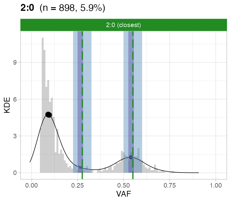
#>
#> [[2]]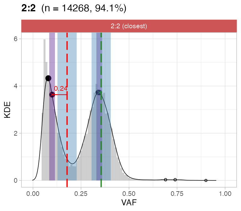
We do the same for a low-cellularity one.
# Low cellularity solution sequenza  (bad calls)
Sequenza_bad_calls = load_SQ_output(Sequenza_URL, sample = 'Set6_42', run = 'lowcell')

# CNA segments and purity
cna = Sequenza_bad_calls$segments
purity = Sequenza_bad_calls$purity

# CNAqc data object
x = CNAqc::init(
  mutations = snvs,
  cna = cna,
  purity = purity,
  ref = "GRCh38") %>%
  CNAqc::analyze_peaks(matching_strategy = 'closest')
#>
#> ── CNAqc - CNA Quality Check ───────────────────────────────────────────────────
#> ℹ Using reference genome coordinates for: GRCh38.
#> ✔ Fortified calls for 18858 somatic mutations: 18858 SNVs (100%) and 0 indels.
#> ! CNAs have no CCF, assuming clonal CNAs (CCF = 1).
#> ! Added segments length (in basepairs) to CNA segments.
#> ✔ Fortified CNAs for 56 segments: 56 clonal and 0 subclonal.
#> ✔ 17283 mutations mapped to clonal CNAs.
#>
#> ── Peak analysis: simple CNAs ──────────────────────────────────────────────────
#> ℹ Analysing 17283 mutations mapping to karyotype(s) 1:0, 1:1, 2:0, and 2:1.
#> ℹ Mixed type peak detection for karyotype 1:0 (898 mutations)
#> ℹ Mixed type peak detection for karyotype 1:1 (14268 mutations)
#> ℹ Mixed type peak detection for karyotype 2:0 (1772 mutations)
#> ℹ Mixed type peak detection for karyotype 2:1 (345 mutations)
#> # A tibble: 6 × 16
#> # Rowwise:
#>   mutation_multiplicity karyotype  peak delta_vaf     x     y counts_per_bin
#>                   <dbl> <chr>     <dbl>     <dbl> <dbl> <dbl>          <int>
#> 1                     1 1:0       0.429    0.0510 0.54  1.26              13
#> 2                     1 1:1       0.3      0.025  0.34  3.73             499
#> 3                     1 2:0       0.3      0.025  0.333 1.30              23
#> 4                     2 2:0       0.6      0.05   0.645 0.497             15
#> 5                     1 2:1       0.231    0.0148 0.277 1.56               5
#> 6                     2 2:1       0.462    0.0296 0.513 0.602              2
#> # ℹ 9 more variables: discarded <lgl>, from <chr>, offset_VAF <dbl>,
#> #   offset <dbl>, weight <dbl>, epsilon <dbl>, VAF_tolerance <dbl>,
#> #   matched <lgl>, QC <chr>
#> ✔ Peak detection PASS with r = -0.087721874571214 - maximum purity error ε = 0.05.
#> Joining with `by = join_by(Major, minor)`
#> Joining with `by = join_by(karyotype)`
#>
#> ── Peak analysis: complex CNAs
#> ─────────────────────────────────────────────────
#> ℹ No karyotypes with >100 mutation(s).
#>
#> ── Peak analysis: subclonal CNAs ───────────────────────────────────────────────
#> ℹ No subclonal CNAs in this sample.

print(x)
#> ── [ CNAqc ] MySample 17283 mutations in 56 segments (56 clonal, 0 subclonal). G
#>
#> ── Clonal CNAs
#>
#>  1:1  [n = 14268, L =  2321 Mb] ■■■■■■■■■■■■■■■■■■■■■■■■■■■
#>  2:0  [n =  1772, L =   277 Mb] ■■■
#>  1:0  [n =   898, L =   141 Mb] ■■
#>  2:1  [n =   345, L =    43 Mb] ■
#> ℹ Sample Purity: 60% ~ Ploidy: 2.
#>
#> ──  PASS  Peaks QC closest: 103%, λ = -0.0877. Purity correction: -9%. ─────────
#> ℹ 1:0 ~ n = 898   (  5%) →  FAIL  -0.094
#> ℹ 1:1 ~ n = 14268 ( 83%) →  PASS  -0.08
#> ℹ 2:0 ~ n = 1772  ( 10%) →  PASS  -0.066   PASS  -0.045
#> ℹ 2:1 ~ n = 345   (  2%) →  FAIL  -0.178   FAIL  -0.093
For this sample these calls are flagged by CNAqc because the purity
is off by a ~10% factor.
plot_peaks_analysis(x, empty_plot = FALSE, assembly_plot = FALSE)
#> [[1]]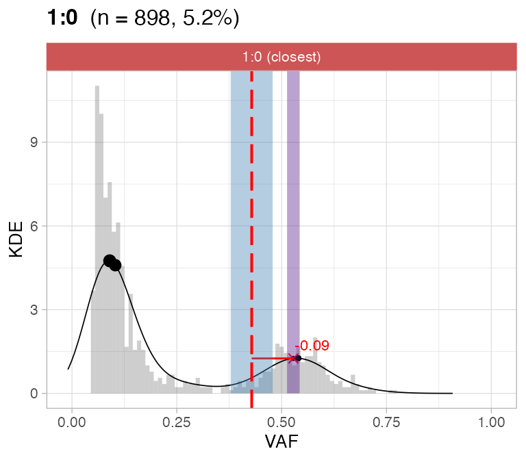
#>
#> [[2]]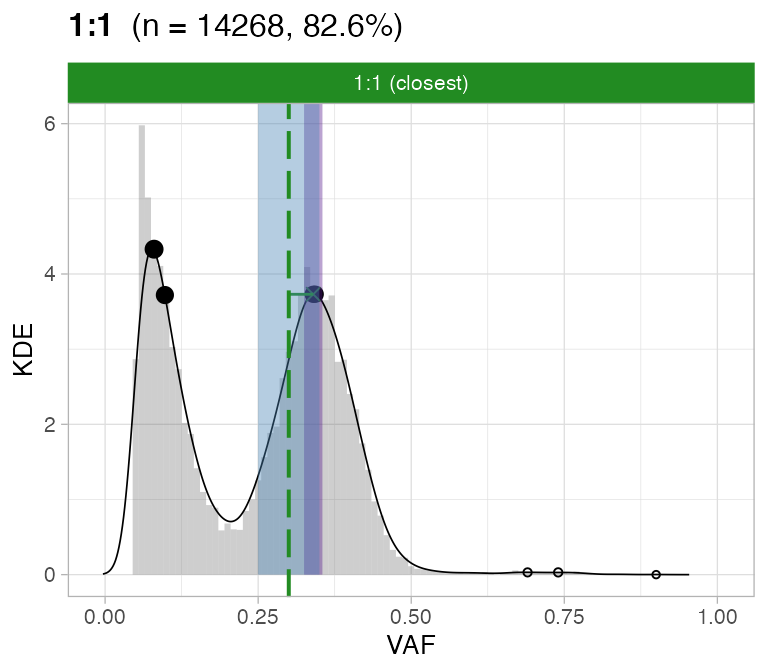
#>
#> [[3]]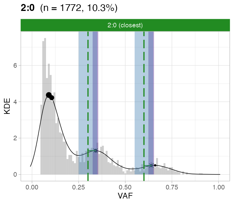
#>
#> [[4]]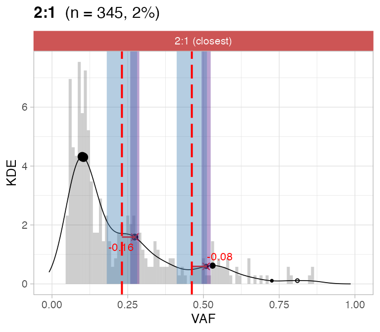
CNAqc can help increasing the caller purity in this case; the
expected adjustment (score from VAF analysis) of 5% would correspond
indeed to a purity increase of 10%.
print(Sequenza_bad_calls$purity - Sequenza_good_calls$purity) # error in these calls
#> [1] -0.09

#CNAqc suggested adjustment
x$peaks_analysis$score
#> [1] -0.08772187