library(CNAqc)
#> ✔ Loading CNAqc, 'Copy Number Alteration quality check'. Support : <https://caravagn.github.io/CNAqc/>

# We work with the PCAWG object
x = CNAqc::example_PCAWG

print(x)
#> ── [ CNAqc ]  293736 mutations in 667 segments (654 clonal, 13 subclonal). Genom
#>
#> ── Clonal CNAs
#>
#>   2:1  [n = 88422, L =   692 Mb] ■■■■■■■■■■■■■■■■■■■■■■■■■■■
#>   3:2  [n = 58384, L =   417 Mb] ■■■■■■■■■■■■■■■■■■  { BRAF }
#>   3:1  [n = 48704, L =   380 Mb] ■■■■■■■■■■■■■■■
#>   3:0  [n = 26622, L =   360 Mb] ■■■■■■■■  { CDKN2A }
#>   2:2  [n = 25290, L =   253 Mb] ■■■■■■■■
#>   3:3  [n = 16790, L =   115 Mb] ■■■■■
#>   2:0  [n =  5374, L =    67 Mb] ■■
#>   4:0  [n =  1752, L =    22 Mb] ■  { TP53 }
#>   4:2  [n =  1441, L =    11 Mb]
#>   1:1  [n =   855, L =     9 Mb]
#>
#> ── Subclonal CNAs (showing up to 10 segments)
#>
#>  chr11@55700000  [n =  10468, L =  78.75 Mb]   2:1 (0.21)   2:2 (0.79) ■■■■■■■■■■
#>  chr11@17365005  [n =   5389, L =  31.55 Mb]   2:1 (0.21)   2:2 (0.79) ■■■■■
#>   chr11@5372292  [n =   1014, L =  11.99 Mb]   2:1 (0.21)   2:2 (0.79)
#>    chr11@202253  [n =    610, L =   5.17 Mb]   2:1 (0.22)   2:2 (0.78)
#>  chr11@48918601  [n =    542, L =   2.68 Mb]   2:1 (0.25)   2:2 (0.75)
#>   chr6@82432583  [n =    301, L =   1.81 Mb]   2:1 (0.19)   2:2 (0.81)
#>  chr11@51600000  [n =    290, L =    4.1 Mb]   2:1 (0.26)   2:2 (0.74)
#>   chr6@81896364  [n =     69, L =   0.54 Mb]   2:1 (0.19)   2:2 (0.81)
#>   chr6@93956180  [n =     41, L =   0.11 Mb]    2:1 (0.2)    2:2 (0.8)
#>   chr8@42633277  [n =     13, L =   0.26 Mb]   2:1 (0.28)   2:2 (0.72)
#> ℹ Sample Purity: 73.4% ~ Ploidy: 3.
#> ℹ There are 3 annotated driver(s) mapped to clonal CNAs.
#>          chr      from        to ref alt DP NV       VAF driver_label is_driver
#>        chr17   7577082   7577082   C   T 78 70 0.8974359         TP53      TRUE
#>         chr7 140453136 140453136   A   T 95 54 0.5684211         BRAF      TRUE
#>         chr9  21971120  21971120   G   A 23 14 0.6086957       CDKN2A      TRUE
#>
#> ──  PASS  Peaks QC closest: 199%, λ = 0.0059. Purity correction: 1%. ───────────
#> ℹ 2:1 ~ n = 88422 ( 74%) →  PASS  0.01     PASS  -0.006
#> ℹ 2:2 ~ n = 25290 ( 21%) →  PASS  0.01     PASS  0.002
#> ℹ 2:0 ~ n = 5374  (  4%) →  PASS  0.015    PASS  -0.001
#> ℹ 1:1 ~ n = 855   (0.7%) →  PASS  -0.006
#> ℹ 1:0 ~ n = 124   (0.1%) →  PASS  0.008
#>
#> ── General peak QC (154430 mutations):  PASS  27  FAIL  13 - epsilon = 0.05. ───
#> ℹ 3:0 ~ n = 26622 ( 17%) →  PASS  3  FAIL  0
#> ℹ 3:1 ~ n = 48704 ( 32%) →  PASS  3  FAIL  0
#> ℹ 3:2 ~ n = 58384 ( 38%) →  PASS  3  FAIL  0
#> ℹ 3:3 ~ n = 16790 ( 11%) →  PASS  3  FAIL  0
#> ℹ 4:2 ~ n = 1441  (  1%) →  PASS  3  FAIL  1
#> ℹ 4:3 ~ n = 359   (  0%) →  PASS  3  FAIL  1
#> ℹ 5:3 ~ n = 132   (  0%) →  PASS  3  FAIL  2
#> ℹ 4:0 ~ n = 1752  (  1%) →  PASS  2  FAIL  2
#> ℹ 5:2 ~ n = 132   (  0%) →  PASS  2  FAIL  3
#> ℹ 6:3 ~ n = 114   (  0%) →  PASS  2  FAIL  4
#>
#> ── Subclonal peaks QC (7 segments, initial state 2:1): linear 5 branching 0 eith
#>
#> ──  PASS  Linear models
#> ℹ chr11@17365005 ~ (31.6Mb, n = 5389) 2:1 (21) + 2:2 (79) : A1B1 -> A1A2B1 -> A1A2B1B2 [100]
#> ℹ   chr11@202253 ~ (5.2Mb, n = 610) 2:1 (22) + 2:2 (78) : A1B1 -> A1A2B1 -> A1A2B1B2 [100]
#> ℹ chr11@51600000 ~ (4.1Mb, n = 290) 2:1 (26) + 2:2 (74) : A1B1 -> A1A2B1 -> A1A2B1B2 [75]
#> ℹ  chr11@5372292 ~ (12Mb, n = 1014) 2:1 (21) + 2:2 (79) : A1B1 -> A1A2B1 -> A1A2B1B2 [100]
#> ℹ chr11@55700000 ~ (78.8Mb, n = 10468) 2:1 (21) + 2:2 (79) : A1B1 -> A1A2B1 -> A1A2B1B2 [100]
#>
#> ──  UNKNOWN  Either branching or linear models
#> ℹ chr11@48918601 ~ (2.7Mb, n = 542) 2:1 (25) + 2:2 (75) : A1B1 -> A1A2B1 -> A1A2B1B2 [100]; A1B1 -> A1A2B1 | A1A2B1B2 [100]; A1B1 -> A1A2B1B2 -> A2B1B2 [100]
#> ℹ  chr6@82432583 ~ (1.8Mb, n = 301) 2:1 (19) + 2:2 (81) : A1B1 -> A1A2B1 -> A1A2B1B2 [100]; A1B1 -> A1A2B1 | A1A2B1B2 [100]; A1B1 -> A1A2B1B2 -> A2B1B2 [100]
#> ✔ Cancer Cell Fraction (CCF) data available for karyotypes:1:0, 1:1, 2:0, 2:1, and 2:2.
#> ✔  PASS  CCF via ENTROPY.
#> ✔  PASS  CCF via ENTROPY.
#> ✔  PASS  CCF via ENTROPY.
#> ✔  PASS  CCF via ENTROPY.
#> ✔  PASS  CCF via ENTROPY.
Peak analysis
CNAqc uses peak-detection algorithms to QC data; all leverage the idea that VAFs peaks are known for mutations mapped to a segment with given minor/ major allele copies. CNAqc therefore computes expected peaks, and compares them to peaks detected from data. The theory works with minor modifications for both clonal and subclonal segments.
Three distinct algorithms are available, each one working with a
different type of copy number segment; all analyses are called by
function analyze_peaks.
x = analyze_peaks(x)
#>
#> ── Peak analysis: simple CNAs ──────────────────────────────────────────────────
#> ℹ Analysing 120065 mutations mapping to karyotype(s) 1:0, 1:1, 2:0, 2:1, and 2:2.
#> ℹ Mixed type peak detection for karyotype 1:0 (124 mutations)
#> ✔ Loading BMix, 'Binomial and Beta-Binomial univariate mixtures'. Support : <https://caravagnalab.github.io/BMix/>
#> ℹ Mixed type peak detection for karyotype 1:1 (855 mutations)
#> ℹ Mixed type peak detection for karyotype 2:0 (5374 mutations)
#> ℹ Mixed type peak detection for karyotype 2:1 (88422 mutations)
#> ℹ Mixed type peak detection for karyotype 2:2 (25290 mutations)
#> # A tibble: 8 × 16
#> # Rowwise:
#>   mutation_multiplicity karyotype  peak delta_vaf     x     y counts_per_bin
#>                   <dbl> <chr>     <dbl>     <dbl> <dbl> <dbl>          <int>
#> 1                     1 1:0       0.580   0.0624  0.570 4.16               7
#> 2                     1 1:1       0.367   0.025   0.366 2.42              15
#> 3                     1 2:0       0.367   0.025   0.359 0.864             50
#> 4                     2 2:0       0.734   0.05    0.735 5.43             265
#> 5                     1 2:1       0.268   0.0134  0.264 4.13            3138
#> 6                     2 2:1       0.537   0.0268  0.54  2.99            2729
#> 7                     1 2:2       0.212   0.00831 0.21  0.93             198
#> 8                     2 2:2       0.423   0.0166  0.423 6.84            1732
#> # ℹ 9 more variables: discarded <lgl>, from <chr>, offset_VAF <dbl>,
#> #   offset <dbl>, weight <dbl>, epsilon <dbl>, VAF_tolerance <dbl>,
#> #   matched <lgl>, QC <chr>
#> ✔ Peak detection PASS with r = 0.0111491116404975 - maximum purity error ε = 0.05.
#> Joining with `by = join_by(Major, minor, QC_PASS)`
#> Joining with `by = join_by(karyotype, QC_PASS)`
#>
#> ── Peak analysis: complex CNAs
#> ─────────────────────────────────────────────────
#> ℹ Karyotypes 3:0, 3:1, 3:2, 3:3, 4:0, 4:2, 4:3, 5:2, 5:3, and 6:3 with >100 mutation(s). Using epsilon = 0.05.
#> # A tibble: 10 × 5
#> # Groups:   karyotype, matched [10]
#>    karyotype     n matched mismatched  prop
#>    <chr>     <int>   <int>      <dbl> <dbl>
#>  1 3:0       26622       3          0 1
#>  2 3:1       48704       3          0 1
#>  3 3:2       58384       3          0 1
#>  4 3:3       16790       3          0 1
#>  5 4:0        1752       3          1 0.75
#>  6 4:2        1441       3          1 0.75
#>  7 4:3         359       3          1 0.75
#>  8 5:3         132       3          2 0.6
#>  9 5:2         132       2          3 0.4
#> 10 6:3         114       2          4 0.333
#> Adding missing grouping variables: `matched`
#> Joining with `by = join_by(Major, minor, QC_PASS, matched)`
#> Adding missing grouping variables: `matched`
#> Joining with `by = join_by(karyotype, QC_PASS, matched)`
#>
#> ── Peak analysis: subclonal CNAs
#> ───────────────────────────────────────────────
#> → Computing evolution models for subclonal CNAs - starting from 1:1
#> # A tibble: 11 × 6
#>    segment_id     model_id                   model      prop size         clones
#>    <chr>          <chr>                      <chr>     <dbl> <chr>        <chr>
#>  1 chr6@82432583  A1B1 -> A1A2B1 -> A1A2B1B2 linear     1    (1.8Mb, n =… 2:1 0…
#>  2 chr6@82432583  A1B1 -> A1A2B1 | A1A2B1B2  branching  1    (1.8Mb, n =… 2:1 0…
#>  3 chr6@82432583  A1B1 -> A1A2B1B2 -> A2B1B2 linear     1    (1.8Mb, n =… 2:1 0…
#>  4 chr11@202253   A1B1 -> A1A2B1 -> A1A2B1B2 linear     1    (5.2Mb, n =… 2:1 0…
#>  5 chr11@5372292  A1B1 -> A1A2B1 -> A1A2B1B2 linear     1    (12Mb, n = … 2:1 0…
#>  6 chr11@17365005 A1B1 -> A1A2B1 -> A1A2B1B2 linear     1    (31.6Mb, n … 2:1 0…
#>  7 chr11@48918601 A1B1 -> A1A2B1 -> A1A2B1B2 linear     1    (2.7Mb, n =… 2:1 0…
#>  8 chr11@48918601 A1B1 -> A1A2B1 | A1A2B1B2  branching  1    (2.7Mb, n =… 2:1 0…
#>  9 chr11@48918601 A1B1 -> A1A2B1B2 -> A2B1B2 linear     1    (2.7Mb, n =… 2:1 0…
#> 10 chr11@51600000 A1B1 -> A1A2B1 -> A1A2B1B2 linear     0.75 (4.1Mb, n =… 2:1 0…
#> 11 chr11@55700000 A1B1 -> A1A2B1 -> A1A2B1B2 linear     1    (78.8Mb, n … 2:1 0…

# Shows results
print(x)
#> ── [ CNAqc ]  293736 mutations in 667 segments (654 clonal, 13 subclonal). Genom
#>
#> ── Clonal CNAs
#>
#>   2:1  [n = 88422, L =   692 Mb] ■■■■■■■■■■■■■■■■■■■■■■■■■■■
#>   3:2  [n = 58384, L =   417 Mb] ■■■■■■■■■■■■■■■■■■  { BRAF }
#>   3:1  [n = 48704, L =   380 Mb] ■■■■■■■■■■■■■■■
#>   3:0  [n = 26622, L =   360 Mb] ■■■■■■■■  { CDKN2A }
#>   2:2  [n = 25290, L =   253 Mb] ■■■■■■■■
#>   3:3  [n = 16790, L =   115 Mb] ■■■■■
#>   2:0  [n =  5374, L =    67 Mb] ■■
#>   4:0  [n =  1752, L =    22 Mb] ■  { TP53 }
#>   4:2  [n =  1441, L =    11 Mb]
#>   1:1  [n =   855, L =     9 Mb]
#>
#> ── Subclonal CNAs (showing up to 10 segments)
#>
#>  chr11@55700000  [n =  10468, L =  78.75 Mb]   2:1 (0.21)   2:2 (0.79) ■■■■■■■■■■
#>  chr11@17365005  [n =   5389, L =  31.55 Mb]   2:1 (0.21)   2:2 (0.79) ■■■■■
#>   chr11@5372292  [n =   1014, L =  11.99 Mb]   2:1 (0.21)   2:2 (0.79)
#>    chr11@202253  [n =    610, L =   5.17 Mb]   2:1 (0.22)   2:2 (0.78)
#>  chr11@48918601  [n =    542, L =   2.68 Mb]   2:1 (0.25)   2:2 (0.75)
#>   chr6@82432583  [n =    301, L =   1.81 Mb]   2:1 (0.19)   2:2 (0.81)
#>  chr11@51600000  [n =    290, L =    4.1 Mb]   2:1 (0.26)   2:2 (0.74)
#>   chr6@81896364  [n =     69, L =   0.54 Mb]   2:1 (0.19)   2:2 (0.81)
#>   chr6@93956180  [n =     41, L =   0.11 Mb]    2:1 (0.2)    2:2 (0.8)
#>   chr8@42633277  [n =     13, L =   0.26 Mb]   2:1 (0.28)   2:2 (0.72)
#> ℹ Sample Purity: 73.4% ~ Ploidy: 3.
#> ℹ There are 3 annotated driver(s) mapped to clonal CNAs.
#>          chr      from        to ref alt DP NV       VAF driver_label is_driver
#>        chr17   7577082   7577082   C   T 78 70 0.8974359         TP53      TRUE
#>         chr7 140453136 140453136   A   T 95 54 0.5684211         BRAF      TRUE
#>         chr9  21971120  21971120   G   A 23 14 0.6086957       CDKN2A      TRUE
#>
#> ──  PASS  Peaks QC closest: 199%, λ = 0.0111. Purity correction: 1%. ───────────
#> ℹ 1:0 ~ n = 124   (0.1%) →  PASS  0.008
#> ℹ 1:1 ~ n = 855   (0.7%) →  PASS  0.002
#> ℹ 2:0 ~ n = 5374  (  4%) →  PASS  0.015    PASS  -0.001
#> ℹ 2:1 ~ n = 88422 ( 74%) →  PASS  0.017    PASS  -0.006
#> ℹ 2:2 ~ n = 25290 ( 21%) →  PASS  0.01     PASS  0.002
#>
#> ── General peak QC (154430 mutations):  PASS  28  FAIL  12 - epsilon = 0.05. ───
#> ℹ 3:0 ~ n = 26622 ( 17%) →  PASS  3  FAIL  0
#> ℹ 3:1 ~ n = 48704 ( 32%) →  PASS  3  FAIL  0
#> ℹ 3:2 ~ n = 58384 ( 38%) →  PASS  3  FAIL  0
#> ℹ 3:3 ~ n = 16790 ( 11%) →  PASS  3  FAIL  0
#> ℹ 4:0 ~ n = 1752  (  1%) →  PASS  3  FAIL  1
#> ℹ 4:2 ~ n = 1441  (  1%) →  PASS  3  FAIL  1
#> ℹ 4:3 ~ n = 359   (  0%) →  PASS  3  FAIL  1
#> ℹ 5:3 ~ n = 132   (  0%) →  PASS  3  FAIL  2
#> ℹ 5:2 ~ n = 132   (  0%) →  PASS  2  FAIL  3
#> ℹ 6:3 ~ n = 114   (  0%) →  PASS  2  FAIL  4
#>
#> ── Subclonal peaks QC (7 segments, initial state 2:1): linear 5 branching 0 eith
#>
#> ──  PASS  Linear models
#> ℹ chr11@17365005 ~ (31.6Mb, n = 5389) 2:1 (21) + 2:2 (79) : A1B1 -> A1A2B1 -> A1A2B1B2 [100]
#> ℹ   chr11@202253 ~ (5.2Mb, n = 610) 2:1 (22) + 2:2 (78) : A1B1 -> A1A2B1 -> A1A2B1B2 [100]
#> ℹ chr11@51600000 ~ (4.1Mb, n = 290) 2:1 (26) + 2:2 (74) : A1B1 -> A1A2B1 -> A1A2B1B2 [75]
#> ℹ  chr11@5372292 ~ (12Mb, n = 1014) 2:1 (21) + 2:2 (79) : A1B1 -> A1A2B1 -> A1A2B1B2 [100]
#> ℹ chr11@55700000 ~ (78.8Mb, n = 10468) 2:1 (21) + 2:2 (79) : A1B1 -> A1A2B1 -> A1A2B1B2 [100]
#>
#> ──  UNKNOWN  Either branching or linear models
#> ℹ chr11@48918601 ~ (2.7Mb, n = 542) 2:1 (25) + 2:2 (75) : A1B1 -> A1A2B1 -> A1A2B1B2 [100]; A1B1 -> A1A2B1 | A1A2B1B2 [100]; A1B1 -> A1A2B1B2 -> A2B1B2 [100]
#> ℹ  chr6@82432583 ~ (1.8Mb, n = 301) 2:1 (19) + 2:2 (81) : A1B1 -> A1A2B1 -> A1A2B1B2 [100]; A1B1 -> A1A2B1 | A1A2B1B2 [100]; A1B1 -> A1A2B1B2 -> A2B1B2 [100]
#> ✔ Cancer Cell Fraction (CCF) data available for karyotypes:1:0, 1:1, 2:0, 2:1, and 2:2.
#> ✔  PASS  CCF via ENTROPY.
#> ✔  PASS  CCF via ENTROPY.
#> ✔  PASS  CCF via ENTROPY.
#> ✔  PASS  CCF via ENTROPY.
#> ✔  PASS  CCF via ENTROPY.
Simple clonal segments (1:0, 2:0,
1:1, 2:1, 2:2)
This QC measures an error for the precision of the current purity estimate, failing a whole sample or a subset of segments the value is over a desired maximum value. The error is determined as a linear combination from the distance between VAF peaks and their theoretical expectation. For this analysis, all mutations mapping across any segment with the same major/minor alleles are pooled.
Note: the score can be used to select among alternative copy number solutions, i.e., favouring a solution with lower score.
The peaks are determined via:
peak-detection algorithms from the peakPick package, applied to a Gaussian kernel density estimate (gKDE) smooth of the VAF distribution;
the Bmix Binomial mixture model.
Peak-matching (i.e., determining what data peak is closest to the expected peak) has two possible implementations:
- one matcheing the closest peaks by euclidean distance;
- the other ranking peaks from higher to lowr VAFs, and prioritising the former.
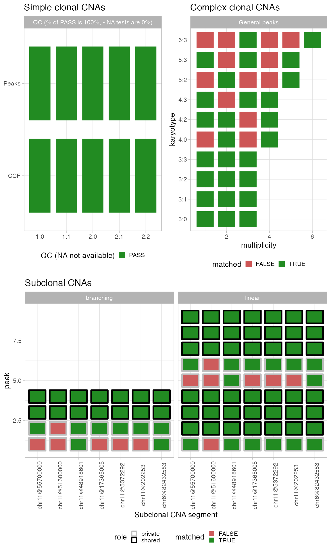
Results from peak-based QC are available via
plot_peaks_analysis.
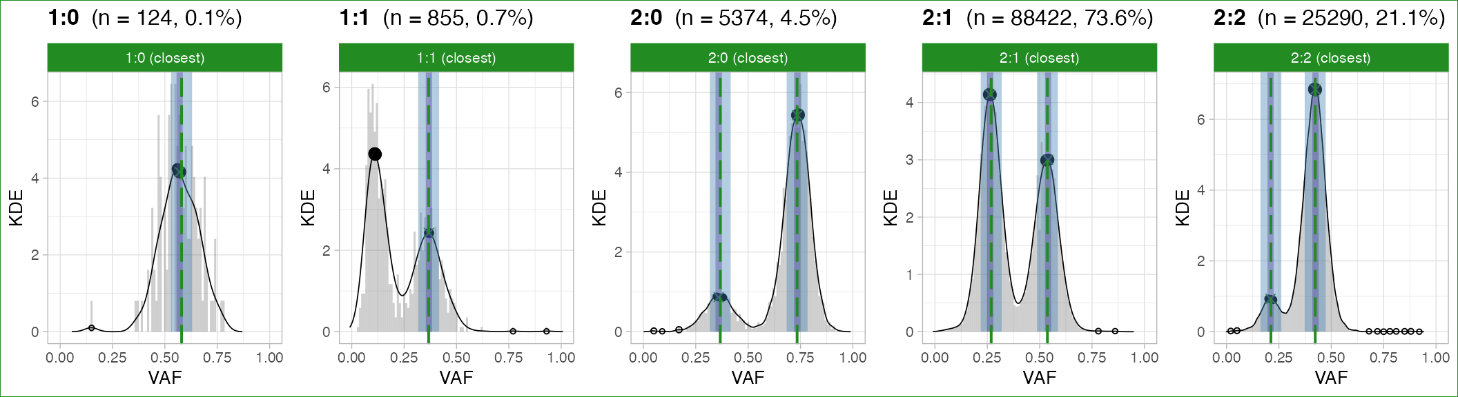
Gray panels are placeholders for segments among 1:0,
2:0, 1:1, 2:1, 2:2
that are not available for the sample. Each vertical dashed line is an
expected peak, the bandwidth around being the tolerance we use to match
peaks (based on purity_error, adjusted for segment ploidy
and tumour purity). Each dot is a peak detected from data, with a
bandwidth of tolerance (fixed) around it.
Note that:
- A green peak is matched, a red one is mismatched;
- The overall segment QC is given by the colour of the facet;
- The overall sample QC is given by the box surrounding the whole figure assembly.
Options of function plot_peaks_analysis allow to
separate the plots.
Note: a chromosome-level analysis is possible by using function
split_by_chromosometo separate a CNAqc object into chromosomes, and then running a standard analysis on each chromosome.
Complex clonal segments
The QC procedure for these “general” segments uses only the gKDE and, as for simple segments, pools all mutations mapping across any segment with the same major/minor alleles.
plot_peaks_analysis(x, what = 'general')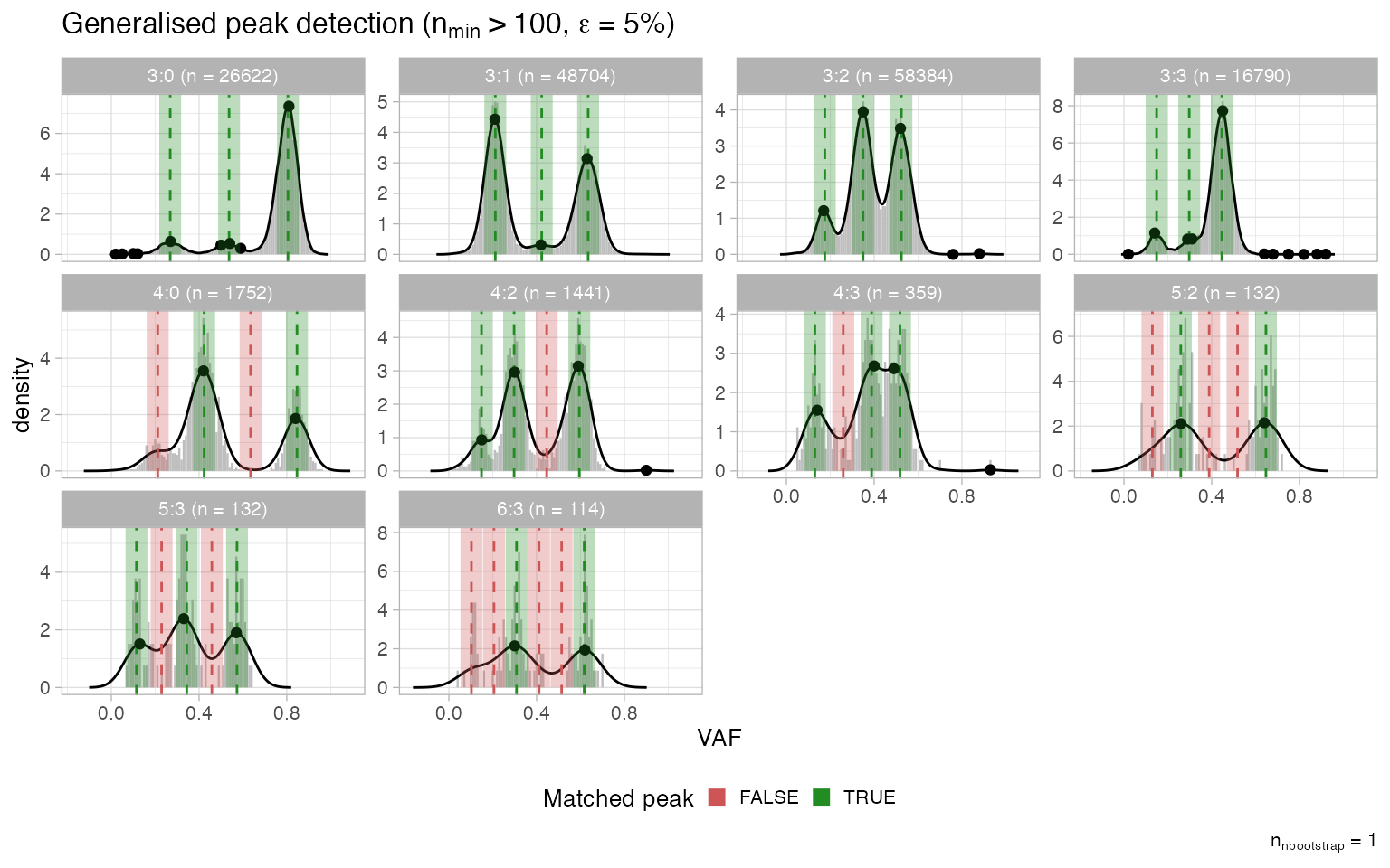
The plot is similar to the one for simple segments, but no segment-level or sample-level scores are produced. A complex segment with many matched peaks is likely to be correct.
Subclonal simple segments
The QC procedure for these segments uses the gKDE and considers 2 subclones with distinct mixing proportions. Differently from clonal CNAs, however, here the analysis is carried out at the level of each segment, i.e., without pooling segments with the same karyotypes. This makes it possible to use subclonal calls fromcallers that report segment-specific CCF values, e.g., Battenberg.
plot_peaks_analysis(x, what = 'subclonal')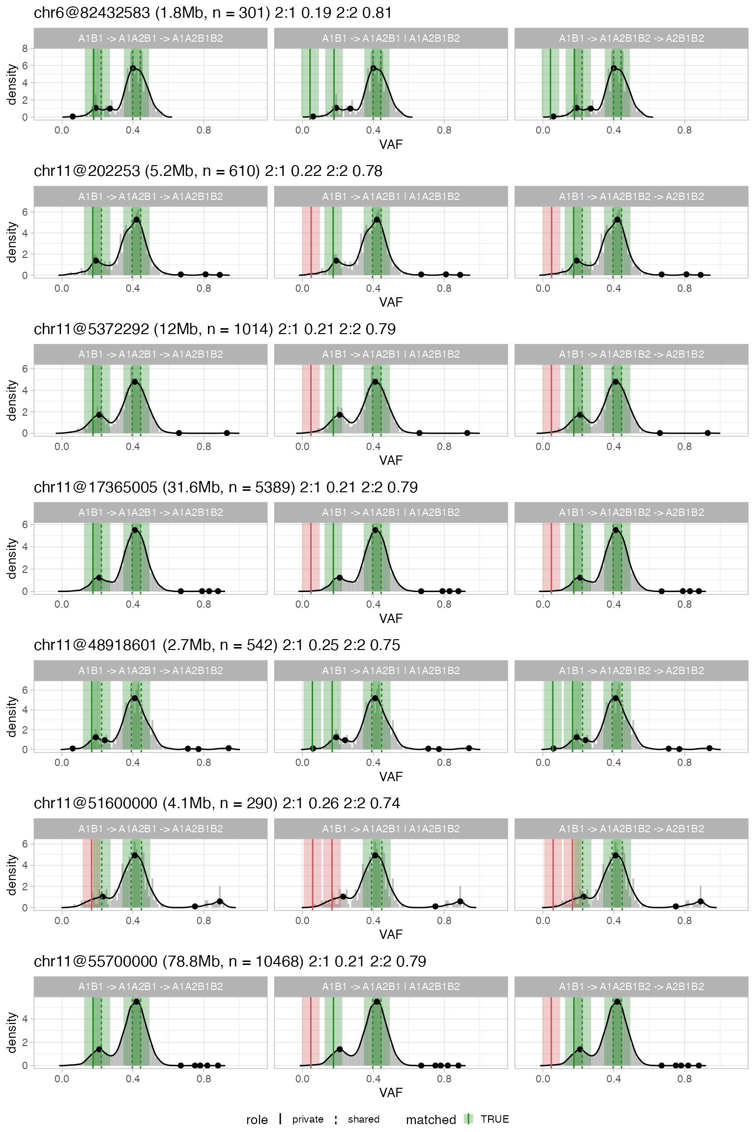 The visual layout of this plot is the same of complex clonal CNAs; not
that the facet reports the distinct evolutionary models that have been
generated to QC subclonal CNAs. The model in CNAqc ranks the proposed
evolutionary alternatives (linear versus branching) based on the number
of matched peaks. A subclonal segment with many matched peaks is likely
to be correct.
The visual layout of this plot is the same of complex clonal CNAs; not
that the facet reports the distinct evolutionary models that have been
generated to QC subclonal CNAs. The model in CNAqc ranks the proposed
evolutionary alternatives (linear versus branching) based on the number
of matched peaks. A subclonal segment with many matched peaks is likely
to be correct.
Summary results
For every type of segment analyzed tables with summary peaks are
available in x$peaks_analysis.
# Simple clonal CNAs - each segment with `discarded = FALSE` has been analysed
x$peaks_analysis$matches
#> # A tibble: 8 × 16
#> # Rowwise:
#>   mutation_multiplicity karyotype  peak delta_vaf     x     y counts_per_bin
#>                   <dbl> <chr>     <dbl>     <dbl> <dbl> <dbl>          <int>
#> 1                     1 1:0       0.580   0.0624  0.570 4.16               7
#> 2                     1 1:1       0.367   0.025   0.366 2.42              15
#> 3                     1 2:0       0.367   0.025   0.359 0.864             50
#> 4                     2 2:0       0.734   0.05    0.735 5.43             265
#> 5                     1 2:1       0.268   0.0134  0.264 4.13            3138
#> 6                     2 2:1       0.537   0.0268  0.54  2.99            2729
#> 7                     1 2:2       0.212   0.00831 0.21  0.93             198
#> 8                     2 2:2       0.423   0.0166  0.423 6.84            1732
#> # ℹ 9 more variables: discarded <lgl>, from <chr>, offset_VAF <dbl>,
#> #   offset <dbl>, weight <dbl>, epsilon <dbl>, VAF_tolerance <dbl>,
#> #   matched <lgl>, QC <chr>

# Complex clonal CNAs
x$peaks_analysis$general$expected_peaks
#> # A tibble: 40 × 9
#>    minor Major ploidy multiplicity purity  peak karyotype matched     n
#>    <dbl> <dbl>  <dbl>        <int>  <dbl> <dbl> <chr>     <lgl>   <int>
#>  1     2     4      6            1  0.734 0.149 4:2       TRUE     1441
#>  2     2     4      6            2  0.734 0.297 4:2       TRUE     1441
#>  3     2     4      6            3  0.734 0.446 4:2       FALSE    1441
#>  4     2     4      6            4  0.734 0.595 4:2       TRUE     1441
#>  5     2     5      7            1  0.734 0.129 5:2       FALSE     132
#>  6     2     5      7            2  0.734 0.259 5:2       TRUE      132
#>  7     2     5      7            3  0.734 0.388 5:2       FALSE     132
#>  8     2     5      7            4  0.734 0.518 5:2       FALSE     132
#>  9     2     5      7            5  0.734 0.647 5:2       TRUE      132
#> 10     0     4      4            1  0.734 0.212 4:0       TRUE     1752
#> # ℹ 30 more rows

# Subclonal CNAs
x$peaks_analysis$subclonal$expected_peaks
#> # A tibble: 91 × 16
#>    mutation karyotype_1 genotype_1 karyotype_2 genotype_2 n.clone_1 n.clone_2
#>    <chr>    <chr>       <chr>      <chr>       <chr>          <int>     <int>
#>  1 HVVBNZKY 2:1         A1A2B1     NA          NA                 1         0
#>  2 LDPZGZTN NA          NA         2:2         A1A2B1B2           0         1
#>  3 XRHVXQJQ 2:1         A1A2B1     2:2         A1A2B1B2           1         2
#>  4 LKZSTZYC 2:1         A1A2B1     2:2         A1A2B1B2           2         2
#>  5 AJSNYKEC NA          NA         2:2         A1A2B1B2           0         1
#>  6 EXPEQGZW 2:1         A1A2B1     2:2         A1A2B1B2           1         1
#>  7 QPTVVSJZ 2:1         A1A2B1     2:2         A1A2B1B2           1         2
#>  8 QKKMNCPT 2:1         A1A2B1     2:2         A1A2B1B2           2         2
#>  9 JINIGKGR NA          NA         2:1         A2B1B2             0         1
#> 10 RJKVCUST 2:2         A1A2B1B2   NA          NA                 1         0
#> # ℹ 81 more rows
#> # ℹ 9 more variables: peak <dbl>, genotype_initial <chr>, model <chr>,
#> #   model_id <chr>, role <chr>, segment_id <chr>, matched <lgl>, size <chr>,
#> #   clones <chr>
The most helpful table is usually the one for simple clonal CNAs
x$peaks_analysis$matches, which reports several
information:
-
mutation_multiplicity, the number of copies of the mutation (i.e., a phasing information); -
peak,x,ythe expected peak, and the matched peak (xandy); -
offset,weightandscore, the factors of the finalscore; -
QC, a"PASS"/"FAIL"status for the peak.
The overall sample-level QC result - "PASS"/"FAIL" - is
available in
x$peaks_analysis$QC
#> [1] "PASS"
You can summarise QC results in a plot.
plot_qc(x)