6. Simulate data

library(dplyr)
n_clocks=3
n_events=8
purity=0.9 
coverage=100 
epsilon=0.20 
seed = 123 
tolerance = 0.0001
max_attempts = 2
INIT = TRUE
min_mutations_number = 3


cat("coverage: ", coverage)

mu = 1e-4 # mutation rate
cat("mutation rate: ", mu)

w = 1e-2 # cell division rate
cat("cell division rate: ", w)

l = 2e7 # length of the segment
cat("length of the segment: ", l)

time_interval = 7
cat("time_interval: ", time_interval)


res_simulate <- tickTack::get_simulation_tickTack(number_clocks=n_clocks, 
                                               number_events=n_events, 
                                               purity=purity, 
                                               coverage=coverage, 
                                               epsilon=epsilon, 
                                               seed = seed)
  
data_simulation = as.data.frame(res_simulate$data_simulation) %>% mutate(chr=   1:length(res_simulate$data_simulation$taus))
x = res_simulate$x

df = x$cna %>% left_join(data_simulation)

# timing inference ticktack hierarchical

x <- tickTack::fit_h(x, max_attempts=max_attempts, INIT=INIT, tolerance = tolerance)


results_simulated <- x$results_timing
results_model_selection <- tickTack::model_selection_h(results_simulated)

## Warning: Some Pareto k diagnostic values are too high. See help('pareto-k-diagnostic') for details.

best_K <- results_model_selection$best_K

data_simulation$taus

## [1] 0.1028646 0.1028646 0.4348927 0.4348927 0.9849570 0.9849570 0.9849570
## [8] 0.4348927

Results

The results object that is returned together with the CNAqc input object contains four components: data, draws_and_summary, log_lik_matrix_list and elbo_iterations.

# View summary for a specific K, here K = 2
results <- x$results

Interpreting the output

We can inspect the main output of interest to understand the timing of clonal peaks. results$draws_and_summary contains: - draws the draws from the approximate posterior distribution of the taus and weights; - summary a summary with the main statistics of the approximate posterior distributions; - summarized_results represents the clock assignment, a tibble with the estimate of taus for each segment with a copy number event that has been included in the hierarchical inference

# View summary for a specific K, here K = 2
results$draws_and_summary[[2]]$summary

## # A tibble: 18 × 7
##    variable    mean  median      sd     mad       q5    q95
##    <chr>      <dbl>   <dbl>   <dbl>   <dbl>    <dbl>  <dbl>
##  1 tau[1]   0.988   0.989   0.00366 0.00318 0.982    0.993 
##  2 tau[2]   0.0925  0.0900  0.0184  0.0181  0.0664   0.125 
##  3 w[1,1]   0.0104  0.00522 0.0180  0.00512 0.000739 0.0367
##  4 w[2,1]   0.00559 0.00230 0.0121  0.00242 0.000268 0.0217
##  5 w[3,1]   0.264   0.259   0.0613  0.0600  0.172    0.371 
##  6 w[4,1]   0.256   0.255   0.0227  0.0232  0.222    0.294 
##  7 w[5,1]   0.996   0.999   0.0102  0.00167 0.984    1.00  
##  8 w[6,1]   0.996   0.998   0.00519 0.00212 0.988    1.00  
##  9 w[7,1]   0.971   0.977   0.0237  0.0150  0.930    0.992 
## 10 w[8,1]   0.249   0.249   0.0268  0.0271  0.205    0.293 
## 11 w[1,2]   0.990   0.995   0.0180  0.00512 0.963    0.999 
## 12 w[2,2]   0.994   0.998   0.0121  0.00242 0.978    1.00  
## 13 w[3,2]   0.736   0.741   0.0613  0.0600  0.629    0.828 
## 14 w[4,2]   0.744   0.745   0.0227  0.0232  0.706    0.778 
## 15 w[5,2]   0.00416 0.00141 0.0102  0.00167 0.000125 0.0159
## 16 w[6,2]   0.00370 0.00212 0.00519 0.00212 0.000263 0.0122
## 17 w[7,2]   0.0292  0.0225  0.0237  0.0150  0.00752  0.0701
## 18 w[8,2]   0.751   0.751   0.0268  0.0271  0.707    0.795

# View detailed summarized results for a specific K, here K = 2
results$draws_and_summary[[2]]$summarized_results

## # A tibble: 8 × 8
##   segment_original_indx segment_name segment_id karyotype   chr clock_mean
##                   <int> <chr>             <dbl> <chr>     <int>      <dbl>
## 1                     1 1_1_2e+07             1 2:1           1     0.0900
## 2                     2 2_1_2e+07             2 2:0           2     0.0900
## 3                     3 3_1_2e+07             3 2:1           3     0.0900
## 4                     4 4_1_2e+07             4 2:2           4     0.0900
## 5                     5 5_1_2e+07             5 2:2           5     0.989 
## 6                     6 6_1_2e+07             6 2:2           6     0.989 
## 7                     7 7_1_2e+07             7 2:1           7     0.989 
## 8                     8 8_1_2e+07             8 2:2           8     0.0900
## # ℹ 2 more variables: clock_low <dbl>, clock_high <dbl>

Obtain the best K with model_selection_h

W e can run the model_selection_h function to obtain the scores for each inference performed with a different K and take the one with best ICL score if the BIC score prefer 2 components instead of 1, otherwise choose 1 as best K. The function takes as input the results and n_components and outputs the best_K and the corresponding best_fit together with the model_selection_tibble and the entropy_list used to evaluate the ICL score.

results_model_selection <- tickTack::model_selection_h(results, n_components = 0)

## Warning: Some Pareto k diagnostic values are too high. See help('pareto-k-diagnostic') for details.

best_K <- results_model_selection$best_K
model_selection_tibble <- results_model_selection$model_selection_tibble
entropy <- results_model_selection$entropy_list
print(best_K)

Visulizing the output

The results can be viewed is genome-wise perspective using the tickTack::plot_timing_h function.

tickTack::plot_timing_h(results, best_K)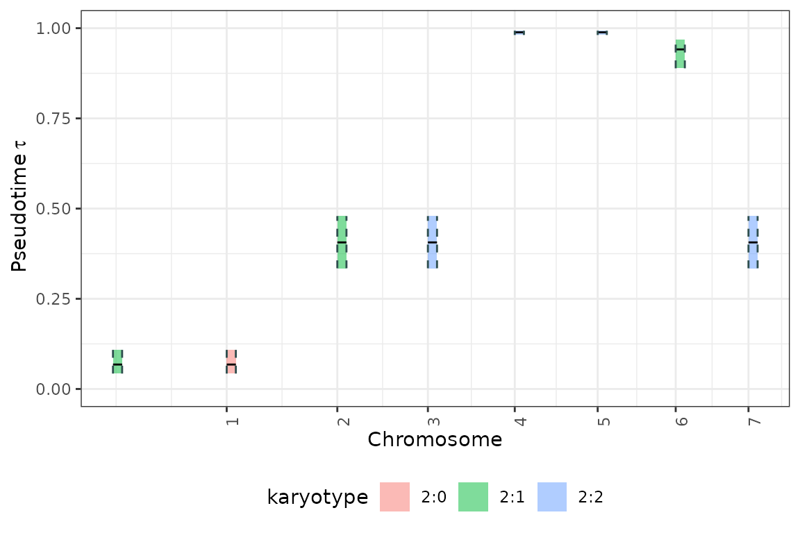

Visualize distributions of draws from the approximate posterior

The approximate posterior distributions can be viewed using the tickTack::plot_posterior_clocks_h and tickTack::plot_posterior_weights_h functions, that internally use functions from Bayesplot.

posterior_clocks <- tickTack::plot_posterior_clocks_h(results, best_K)

## Scale for x is already present.
## Adding another scale for x, which will replace the existing scale.

posterior_weights <- tickTack::plot_posterior_weights_h(results, best_K)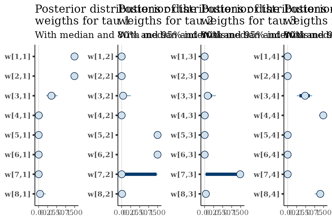

Visualize the behavior of the ELBO during the inference

K = nrow(results_model_selection$model_selection_tibble)

p_elbo <- list()
for (i in 1:K){
  p_elbo[[i]] <- tickTack::plot_elbo_h(results$elbo_iterations[[i]]) + ggplot2::ggtitle(paste0("K = ", i))
}
p_elbo <- gridExtra::grid.arrange(grobs = p_elbo, ncol = 2)  #add global title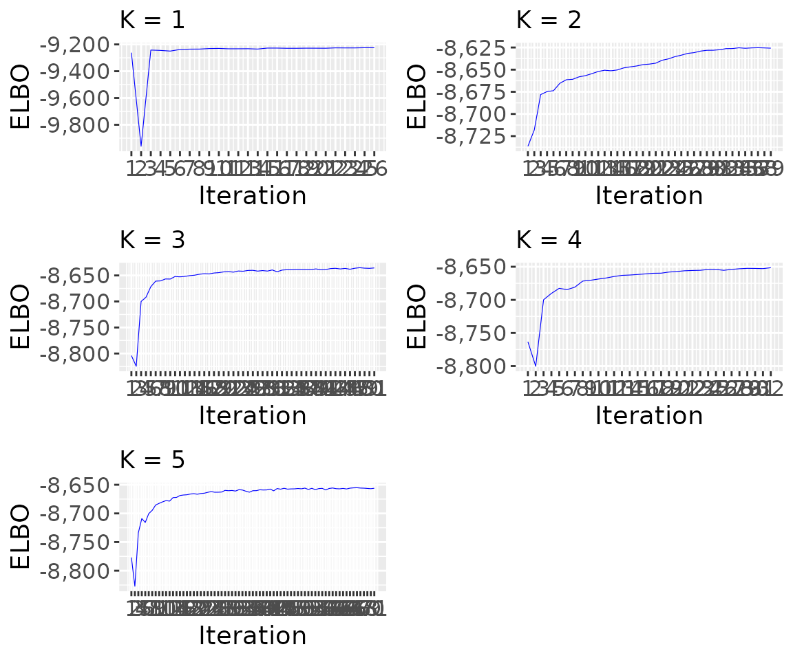

p_elbo

## TableGrob (2 x 2) "arrange": 4 grobs
##   z     cells    name           grob
## 1 1 (1-1,1-1) arrange gtable[layout]
## 2 2 (1-1,2-2) arrange gtable[layout]
## 3 3 (2-2,1-1) arrange gtable[layout]
## 4 4 (2-2,2-2) arrange gtable[layout]

Visualize all the inference results for each K

plot_model_selection_inference <- list()
for (i in 1:K){
  plot_model_selection_inference[[i]] <- tickTack::plot_timing_h(results, i) + ggplot2::ggtitle(paste0("K = ", i))
}
plot_model_selection_inference <- gridExtra::grid.arrange(grobs = plot_model_selection_inference, ncol = 2) #add global title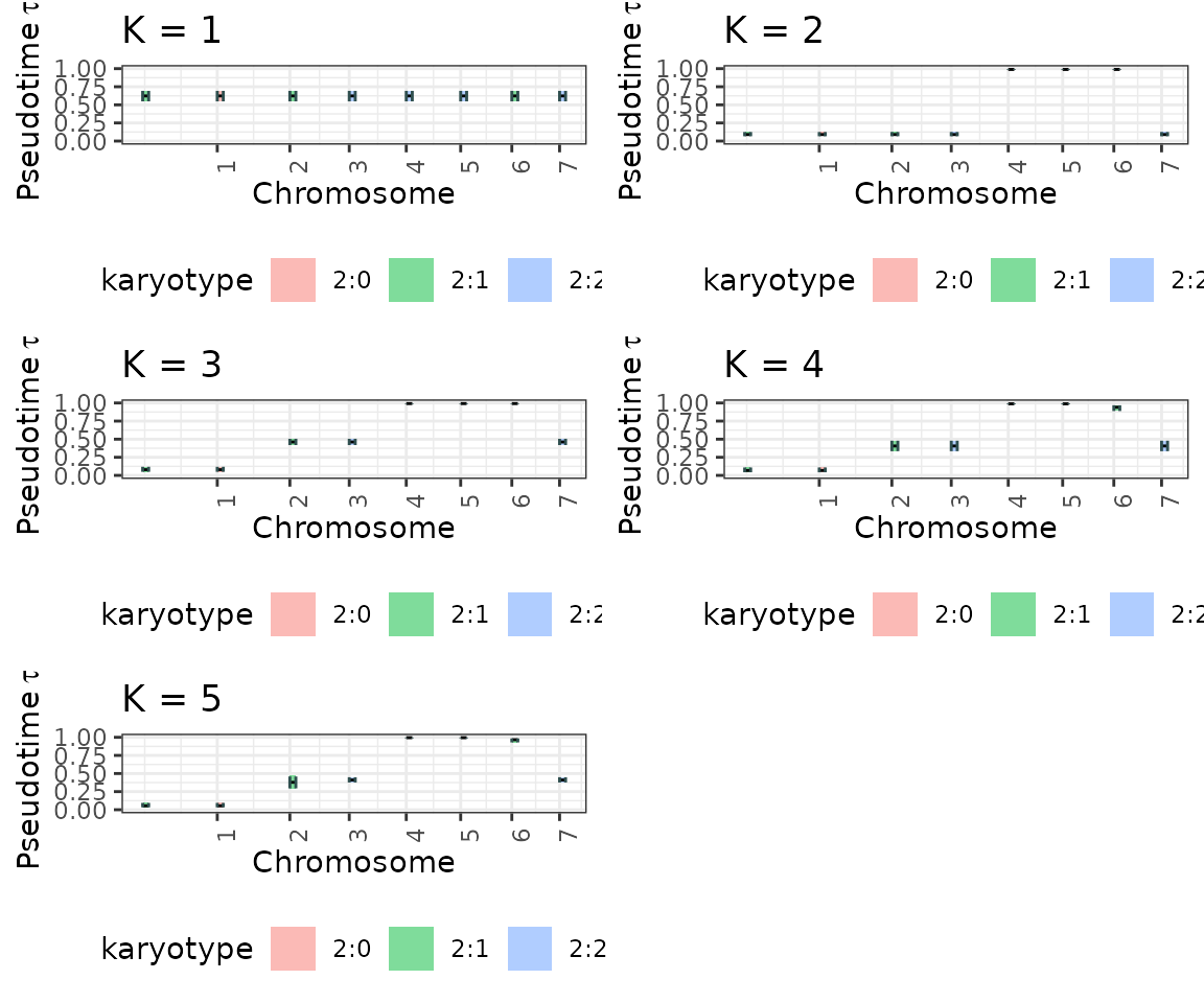

plot_model_selection_inference

## TableGrob (2 x 2) "arrange": 4 grobs
##   z     cells    name           grob
## 1 1 (1-1,1-1) arrange gtable[layout]
## 2 2 (1-1,2-2) arrange gtable[layout]
## 3 3 (2-2,1-1) arrange gtable[layout]
## 4 4 (2-2,2-2) arrange gtable[layout]