4. Timing Clonal Peaks in a hierarchical fashioin
a4_Multiple_segment_timing.RmdThe _fit_h function in the tickTack package
estimates the timing of K clonal binomial peaks in cancer
genome sequencing data according to which a clustering can be performed.
This vignette describes the functionality of the fit_h
function, including input requirements, output, and an example analysis
using the tickTack::pcawg_example_2 dataset.
Overview of the fit_h Function
The fit_h function uses a hierarchical model to fit
clonal binomial peaks in sequencing data considering the grouping
structure of the chromosomes segments. It identifies segments of the
genome with specific karyotypes and mutations that meet the input
criteria, then estimates the timing of the groups of events and assign
each segment to a clock. The clock represents the pseudotime, where 0 is
the moment the cancerous population was born and 1 is the time of the
most recent common ancestor (MRCA) of the cells in the bulk sequencing
sample.
Key Parameters
-
x: a CNAqc object with mutations, cna and metadata -
max_attempts: Number of times the variational inference is repeated to avoid local minima. -
INIT: Logical flag to pass some initialization values tothe variational inference, default isTRURE. -
tolerance: tolerance between two value of subsequent iterations of gradient ascent on elbo, default is0.01. -
possible_k: A character vector of possible karyotypes, defaulting toc("2:1", "2:2", "2:0"). -
alpha: Significance level, defaulting to0.05. -
min_mutations_number: Minimum number of mutations required for analysis, defaulting to2. -
n_components: If0, then the strategy to choose the #components follows the default procedure, otherwise the inference is repeated for K equal up to a maximun of n_components.
Output
The function returns a list containing:
-
data: The data used to perform the inference after selecting the ones that respect the assumptions to be used in the model. -
draws_and_summary: List of 3 for each K the inference is performed with. Draws are available both for the clocks and for the weights Summary statistics for the estimated timing of clonal peaks. -
log_lik_matrix_list: Summary statistics for the estimated timing of clonal peaks. -
elbo_iterations: Summary statistics for the estimated timing of clonal peaks.
If no segments meet the criteria, the function returns
NULL.
Analyzing tickTack::pcawg_example_2
We will use the tickTack::pcawg_example_2 dataset to
demonstrate how to use the fit_h function.
Input Data
The tickTack::pcawg_example_2 dataset contains three
components:
-
mutations: Mutation data. -
cna: Copy number alterations (CNA). -
metadata: Sample metadata, including tumor purity.
Preview the data:
library(tickTack)
library(patchwork)
library(ggplot2)


# View example dataset components
mutations <- tickTack::pcawg_example_2$mutations
cna <- tickTack::pcawg_example_2$cna
metadata <- tickTack::pcawg_example_2$metadata

head(mutations)
## # A tibble: 6 × 45
## chr from to ref alt DP NV VAF sample NR Hugo_Symbol
## <chr> <dbl> <dbl> <chr> <chr> <dbl> <dbl> <dbl> <chr> <dbl> <chr>
## 1 chr1 1018754 1018754 C C 51 24 0.471 3b7810f… 27 C1orf159
## 2 chr1 1107556 1107556 C C 53 17 0.321 3b7810f… 36 TTLL10
## 3 chr1 1127192 1127192 C C 78 13 0.167 3b7810f… 65 TTLL10
## 4 chr1 1255263 1255263 C C 66 23 0.348 3b7810f… 43 CPSF3L
## 5 chr1 1474126 1474126 C C 68 17 0.25 3b7810f… 51 TMEM240
## 6 chr1 1532289 1532289 G G 39 6 0.154 3b7810f… 33 C1orf233
## # ℹ 34 more variables: Strand <chr>, Variant_Classification <chr>,
## # Variant_Type <chr>, Tumor_Seq_Allele2 <chr>, dbSNP_RS <chr>,
## # dbSNP_Val_Status <chr>, Matched_Norm_Sample_Barcode <chr>,
## # Genome_Change <chr>, ref_context <chr>, gc_content <dbl>,
## # i_1000genomes_AF <dbl>, i_1000genomes_ID <chr>, i_Callers <chr>,
## # i_GERM1000G <lgl>, i_GERMOVLP <lgl>, i_LOWSUPPORT <lgl>,
## # i_NORMALPANEL <lgl>, i_NumCallers <dbl>, i_OXOGFAIL <lgl>, …
head(cna)## # A tibble: 6 × 39
## chr from to Major minor CCF total_cn star level methods_agree
## <chr> <dbl> <dbl> <dbl> <dbl> <dbl> <dbl> <dbl> <chr> <dbl>
## 1 chr1 10001 121499999 1 1 1 2 3 a 6
## 2 chr1 121500000 128899999 1 1 1 2 2 d 4
## 3 chr1 128900000 247247500 1 1 1 2 3 a 6
## 4 chr1 247247501 249250620 1 1 1 2 2 d 4
## 5 chr2 66017 90499999 1 1 1 2 3 a 6
## 6 chr2 90500000 96799999 1 1 1 2 3 a 6
## # ℹ 29 more variables: absolute_broad_major_cn <dbl>,
## # absolute_broad_minor_cn <dbl>, absolute_broad_het_error <dbl>,
## # absolute_broad_cov_error <dbl>, aceseq_copy_number <dbl>,
## # aceseq_minor_cn <dbl>, aceseq_major_cn <dbl>, battenberg_nMaj1_A <dbl>,
## # battenberg_nMin1_A <dbl>, battenberg_frac1_A <dbl>,
## # battenberg_nMaj2_A <dbl>, battenberg_nMin2_A <dbl>,
## # battenberg_frac2_A <dbl>, battenberg_SDfrac_A <dbl>, …
metadata## # A tibble: 1 × 6
## sample purity ploidy purity_conf_mad wgd_status wgd_uncertain
## <chr> <dbl> <dbl> <dbl> <chr> <lgl>
## 1 3b7810f7-f8ff-4d62-b76… 0.611 1.92 0.002 no_wgd FALSERunning the fit_h function
We can run the fit_h function on the
tickTack::pcawg_example_2 data to infer the timing of
clonal peaks
Results
The results object that is returned together with the
CNAqc input object contains four components: data,
draws_and_summary, log_lik_matrix_list and
elbo_iterations. In the data there are both
the input_data passed to the Stan model and the
accepted_cna segments that respect the selection conditions
and are included in the inference. The draws_and_summary
part present an object for each inference performed with the used number
of components. Each of them is named by the number of components
K used for the inference so we can access them as
below.
# View results
fit$results_timing$data$accepted_cna
## # A tibble: 10 × 5
## segment_original_indx segment_name segment_id karyotype chr
## <int> <chr> <dbl> <chr> <chr>
## 1 38 chr5_75225353_75780032 1 2:1 chr5
## 2 40 chr5_76857368_76998901 2 2:1 chr5
## 3 42 chr5_77822720_82754991 3 2:1 chr5
## 4 44 chr5_83468190_180689978 4 2:1 chr5
## 5 46 chr6_242501_4335355 5 2:0 chr6
## 6 48 chr6_4347801_29092265 6 2:0 chr6
## 7 50 chr6_29161839_38477499 7 2:0 chr6
## 8 54 chr7_65454_9937168 8 2:1 chr7
## 9 56 chr7_9946564_57999999 9 2:1 chr7
## 10 58 chr7_61700000_158817500 10 2:1 chr7
results <- fit$results_timingInterpreting the output
We can inspect the main output of interest to understand the timing
of clonal peaks. results$draws_and_summary contains: -
draws the draws from the approximate
posterior distribution of the taus and weights; -
summary a summary with the main statistics
of the approximate posterior distributions; -
summarized_results represents the clock
assignment, a tibble with the estimate of taus for each segment with a
copy number event that has been included in the hierarchical
inference
# View summary for a specific K, here K = 1
inference_with_1_component <- results$draws_and_summary[["1"]]
inference_with_5_component <- results$draws_and_summary[["5"]]

# View detailed summarized results for a specific K, here K = 1 and K = 5
inference_with_1_component$summarized_results
## # A tibble: 10 × 10
## segment_original_indx segment_name segment_id karyotype chr clock_mean
## <int> <chr> <dbl> <chr> <chr> <dbl>
## 1 38 chr5_75225353_75… 1 2:1 chr5 0.242
## 2 40 chr5_76857368_76… 2 2:1 chr5 0.242
## 3 42 chr5_77822720_82… 3 2:1 chr5 0.242
## 4 44 chr5_83468190_18… 4 2:1 chr5 0.242
## 5 46 chr6_242501_4335… 5 2:0 chr6 0.242
## 6 48 chr6_4347801_290… 6 2:0 chr6 0.242
## 7 50 chr6_29161839_38… 7 2:0 chr6 0.242
## 8 54 chr7_65454_99371… 8 2:1 chr7 0.242
## 9 56 chr7_9946564_579… 9 2:1 chr7 0.242
## 10 58 chr7_61700000_15… 10 2:1 chr7 0.242
## # ℹ 4 more variables: clock_low <dbl>, clock_high <dbl>, alpha <dbl>,
## # beta <dbl>
inference_with_5_component$summarized_results## # A tibble: 10 × 10
## segment_original_indx segment_name segment_id karyotype chr clock_mean
## <int> <chr> <dbl> <chr> <chr> <dbl>
## 1 38 chr5_75225353_75… 1 2:1 chr5 0.368
## 2 40 chr5_76857368_76… 2 2:1 chr5 0.000612
## 3 42 chr5_77822720_82… 3 2:1 chr5 0.0269
## 4 44 chr5_83468190_18… 4 2:1 chr5 0.0269
## 5 46 chr6_242501_4335… 5 2:0 chr6 0.955
## 6 48 chr6_4347801_290… 6 2:0 chr6 0.955
## 7 50 chr6_29161839_38… 7 2:0 chr6 0.955
## 8 54 chr7_65454_99371… 8 2:1 chr7 0.167
## 9 56 chr7_9946564_579… 9 2:1 chr7 0.167
## 10 58 chr7_61700000_15… 10 2:1 chr7 0.167
## # ℹ 4 more variables: clock_low <dbl>, clock_high <dbl>, alpha <dbl>,
## # beta <dbl>Obtain the best K with model_selection_h
W e can run the model_selection_h function to obtain the
scores for each inference performed with a different K and take the one
with best ICL score if the BIC score prefer 2 components instead of 1,
otherwise choose 1 as best K. The function takes as input the
results and n_components and outputs the
best_K and the corresponding best_fit together
with the model_selection_tibble and the
entropy_list used to evaluate the ICL score.
results_model_selection <- tickTack::model_selection_h(results, n_components = 0)## Warning: Some Pareto k diagnostic values are too high. See help('pareto-k-diagnostic') for details.
## Warning: Some Pareto k diagnostic values are too high. See help('pareto-k-diagnostic') for details.
## Warning: Some Pareto k diagnostic values are too high. See help('pareto-k-diagnostic') for details.
## Warning: Some Pareto k diagnostic values are too high. See help('pareto-k-diagnostic') for details.
best_K <- results_model_selection$best_K
model_selection_tibble <- results_model_selection$model_selection_tibble
Visulizing the output
The results can be viewed is genome-wise perspective using the
tickTack::plot_timing_h function.
# fit$metadata = tibble(purity=fit$purity)
# fit$cna <- fit$cna%>%mutate(Major_2=Major,minor_2=minor)
library(dplyr)
##
## Attaching package: 'dplyr'## The following objects are masked from 'package:stats':
##
## filter, lag## The following objects are masked from 'package:base':
##
## intersect, setdiff, setequal, union
fit$reference_genome <- "GRCh37"
fit$cna <- fit$cna%>%mutate(Major_2=Major,minor_2=minor)
plot_cnaqc(fit,add_mobster=F)
## Warning: Some Pareto k diagnostic values are too high. See help('pareto-k-diagnostic') for details.
## Warning: Some Pareto k diagnostic values are too high. See help('pareto-k-diagnostic') for details.
## Warning: Some Pareto k diagnostic values are too high. See help('pareto-k-diagnostic') for details.
## Warning: Some Pareto k diagnostic values are too high. See help('pareto-k-diagnostic') for details.## ✔ Loading CNAqc, 'Copy Number Alteration quality check'. Support : <https://caravagn.github.io/CNAqc/>## ## ── CNAqc - CNA Quality Check ───────────────────────────────────────────────────## ℹ Using reference genome coordinates for: GRCh37.## ! Detected indels mutation (substitutions with >1 reference/alternative nucleotides).## ✖ NA values in some of the required mutation columns, these will be removed.## ✔ Fortified calls for 41400 somatic mutations: 36223 SNVs (87%) and 5177 indels.## ℹ 2 subclonal CNAs detected in the data.## ! Added segments length (in basepairs) to CNA segments.## ✔ Fortified CNAs for 107 segments: 105 clonal and 2 subclonal.## ✔ 39324 mutations mapped to clonal CNAs.## Warning: Unknown or uninitialised column: `mutations`.## ✔ 0 mutations mapped to subclonal CNAs.## Warning: Using `size` aesthetic for lines was deprecated in ggplot2 3.4.0.
## ℹ Please use `linewidth` instead.
## ℹ The deprecated feature was likely used in the CNAqc package.
## Please report the issue at <https://github.com/caravagnalab/CNAqc/issues>.
## This warning is displayed once per session.
## Call `lifecycle::last_lifecycle_warnings()` to see where this warning was
## generated.## Warning: Removed 17 rows containing missing values or values outside the scale range
## (`geom_segment()`).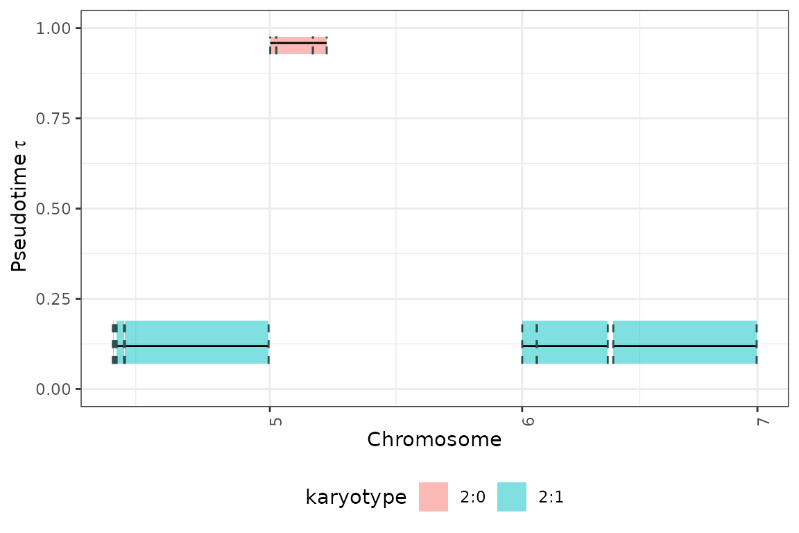
Visualize distributions of draws from the approximate posterior
The approximate posterior distributions can be viewed using the
tickTack::plot_posterior_clocks_h and
tickTack::plot_posterior_weights_h functions, that
internally use functions from Bayesplot.
posterior_clocks <- tickTack::plot_posterior_clocks_h(results, 2)## Scale for x is already present.
## Adding another scale for x, which will replace the existing scale.
posterior_weights <- tickTack::plot_posterior_weights_h(results, 2)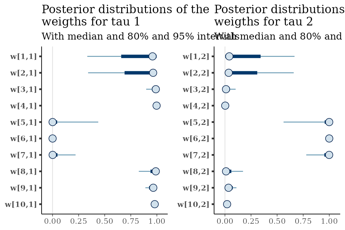
Visualize the behavior of the ELBO during the inference
K = nrow(results_model_selection$model_selection_tibble)

p_elbo <- list()
for (i in 1:K){
  p_elbo[[i]] <- tickTack::plot_elbo_h(results$elbo_iterations[[i]]) + ggplot2::ggtitle(paste0("K = ", i))
}
p_elbo <- gridExtra::grid.arrange(grobs = p_elbo, ncol = 2)  #add global title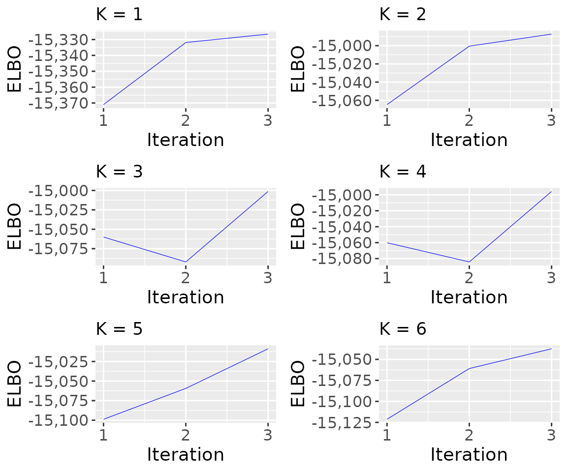
p_elbo## TableGrob (3 x 2) "arrange": 5 grobs
## z cells name grob
## 1 1 (1-1,1-1) arrange gtable[layout]
## 2 2 (1-1,2-2) arrange gtable[layout]
## 3 3 (2-2,1-1) arrange gtable[layout]
## 4 4 (2-2,2-2) arrange gtable[layout]
## 5 5 (3-3,1-1) arrange gtable[layout]Visualize all the inference results for each K
plot_model_selection_inference <- list()
for (i in 1:K){
  plot_model_selection_inference[[i]] <- tickTack::plot_timing_h(results, i) + ggplot2::ggtitle(paste0("K = ", i))
}
plot_model_selection_inference <- gridExtra::grid.arrange(grobs = plot_model_selection_inference, ncol = 2) #add global title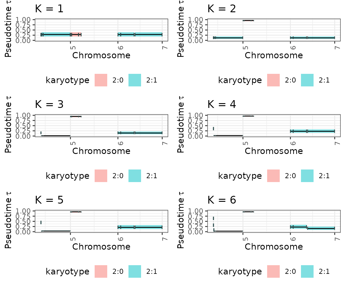
plot_model_selection_inference## TableGrob (3 x 2) "arrange": 5 grobs
## z cells name grob
## 1 1 (1-1,1-1) arrange gtable[layout]
## 2 2 (1-1,2-2) arrange gtable[layout]
## 3 3 (2-2,1-1) arrange gtable[layout]
## 4 4 (2-2,2-2) arrange gtable[layout]
## 5 5 (3-3,1-1) arrange gtable[layout]