1. Introduction

library(mobster)
library(tidyr)
library(dplyr)

Input data for `mobster`

You can run a MOBSTER analysis if, for a set of input mutations (SNVs, indels etc.), you have available VAF or CCF data. The input data can be loaded using different input formats.

For VAF values you can use:

a data.frame (or, tibble) with a column named VAF whose values are numerical $0<x<1$ , without NA entries and columns named any of those: cluster, Tail, C1, C2, C3,…;
a VCF file that must contain at least a column with the total depth of sequencing and the number of reads with the variants. In this case you need first to use function load_VCF and load the VCF content, and then proceed using your data as a data.frame.

For CCF values you can only use the a data.frame format. Importantly, you have to store the CCF values in a column again named VAF, which must follow the same convention of a VAF column (i.e., range of values). Since CCF values usually peak at around 1.0 for clonal mutations (i.e., present in 100% of the input cells), we suggest to adjust standard CCF estimates dividing them by 0.5 in order to reflect the peak of an heterozygous clonal mutation at 50% VAF for a 100% pure bulk sample.

Example dataset. Diploid mutations from sample LU4 of the Comprehensive Omics Archive of Lung Adenocarcinoma are available in the package under the name LU4_lung_sample. The available object is the results of an analysis with mobster, and the input mutation data is stored inside the object.

# Example dataset LU4_lung_sample, downloaded from http://genome.kaist.ac.kr/
print(mobster::LU4_lung_sample$best$data)
#> # A tibble: 1,282 × 12
#>      Key Callers     t_alt_count t_ref_count Variant_Classification    DP    VAF
#>    <int> <chr>             <int>       <int> <chr>                  <int>  <dbl>
#>  1   370 mutect,str…          30          95 intergenic               125 0.24  
#>  2   371 mutect,str…          10         105 intergenic               115 0.0870
#>  3   372 mutect,str…          40         108 intronic                 148 0.270 
#>  4   373 mutect,str…          20         101 intronic                 121 0.165 
#>  5   374 mutect,str…          39          89 intergenic               128 0.305 
#>  6   375 mutect,str…          41         120 intronic                 161 0.255 
#>  7   376 mutect,str…          43          93 intronic                 136 0.316 
#>  8   377 mutect,str…          22          95 intergenic               117 0.188 
#>  9   378 mutect                7         104 intergenic               111 0.0631
#> 10   379 mutect,str…          35          93 intergenic               128 0.273 
#> # ℹ 1,272 more rows
#> # ℹ 5 more variables: chr <chr>, from <chr>, ref <chr>, alt <chr>,
#> #   cluster <chr>

Other datasets are available through the data command.

Driver annotations

In the context of subclonal deconvolution we are often interested in linking “driver” events to clonal expansions. Since mobster works with somatic mutations data, it is possible to annotate the status of “driver mutation” in the input data; doing so, the drivers will be reported in some visualisations of the tool, but will not influence any of the computation carried out in mobster.

The annotate one or more driver mutations you need to include in your column 2 extra columns:

is_driver, a boolean TRUE/FALSE flag;
driver_label, a character string that will be used as label in any visualisation that uses drivers.

Generating random models and data

You can sample a random dataset with the random_dataset function, setting:

the number of mutations (n) and Beta components (k, subclones) to generate;
ranges and constraints on the size of the components;
ranges for the mean and variance of the Beta components.

The variance of the Betas is defined as $u/B$ where $u \sim U[0,1]$ , and $B$ is the input parameter Beta_variance_scaling. Roughly, values of Beta_variance_scaling on the order of 1000 give low variance and sharp peaked data distributions. Values on the order of 100 give much wider distributions.

dataset = random_dataset(
  seed = 123456789, 
  Beta_variance_scaling = 100    # variance ~ U[0, 1]/Beta_variance_scaling
  )

A list with 3 components is returned, which contains the actual data, sampled parameters of the generative model, and a plot of the data.

In mobster we provide the implementation of the model’s density function (ddbpmm, density Dirichlet Beta Pareto mixture model), and a sampler (rdbpmm) which is used internally by random_dataset to generate the data.

# Data, in the MOBSTER input format with a "VAF" column.
print(dataset$data)
#> # A tibble: 5,000 × 2
#>      VAF simulated_cluster
#>    <dbl> <chr>            
#>  1 0.856 C1               
#>  2 0.853 C1               
#>  3 0.844 C1               
#>  4 0.827 C1               
#>  5 0.855 C1               
#>  6 0.854 C1               
#>  7 0.878 C1               
#>  8 0.865 C1               
#>  9 0.845 C1               
#> 10 0.874 C1               
#> # ℹ 4,990 more rows

# The generated model contains the parameters of the Beta components (a and b),
# the shape and scale of the tail, and the mixing proportion. 
print(dataset$model)
#> $a
#>      C1      C2 
#> 72.6286 30.5932 
#> 
#> $b
#>       C1       C2 
#> 13.07363 24.93900 
#> 
#> $shape
#> [1] 1
#> 
#> $scale
#> [1] 0.05
#> 
#> $pi
#>      Tail        C1        C2 
#> 0.3431634 0.3331162 0.3237204

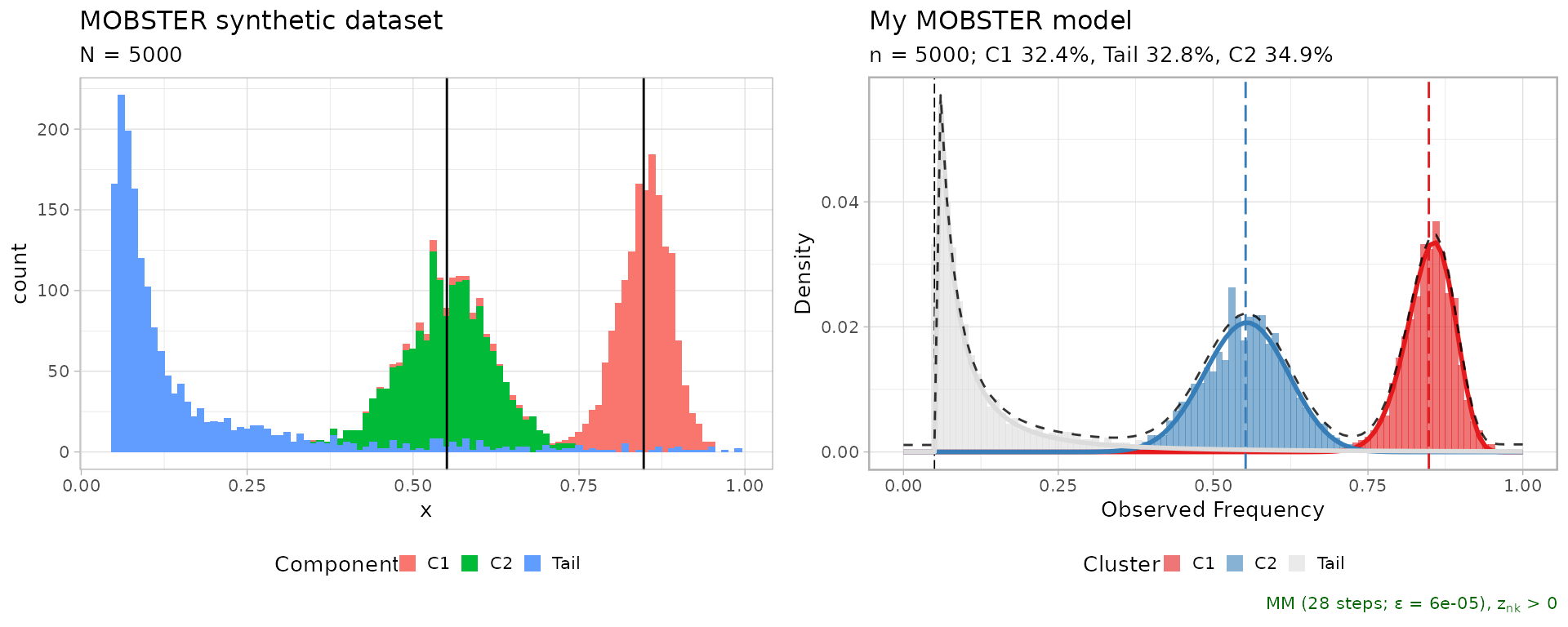
# A plot object (ggplot) is available where each data-point is coloured by 
# its generative mixture component. The vertical lines annontate the means of
# the sampled Beta distributions.
print(dataset$plot)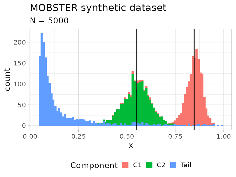

Fitting a dataset

Function mobster_fit fits a MOBSTER model.

The function implements a model-selection routine that by default scores models by their reICL (reduced Integrative Classification Likelihood) score, a variant to the popular BIC that uses the entropy of the latent variables of the mixture. reICL is discussed in the main paper.

This function has several parameters to customize the fitting procedure, and a set of special pre-parametrised runs that can be activated with parameter auto_setup. Here we use auto_setup = "FAST", an automatic setup for a fast run; its parameters are accessible through an internal package function.

# Hidden function (:::)
mobster:::template_parameters_fast_setup()
#> $K
#> [1] 1 2
#> 
#> $samples
#> [1] 2
#> 
#> $init
#> [1] "random"
#> 
#> $tail
#> [1]  TRUE FALSE
#> 
#> $epsilon
#> [1] 1e-06
#> 
#> $maxIter
#> [1] 100
#> 
#> $fit.type
#> [1] "MM"
#> 
#> $seed
#> [1] 12345
#> 
#> $model.selection
#> [1] "reICL"
#> 
#> $trace
#> [1] FALSE
#> 
#> $parallel
#> [1] FALSE
#> 
#> $pi_cutoff
#> [1] 0.02
#> 
#> $N_cutoff
#> [1] 10

Compared to these, default parameters test more extensive types of fits (i.e., more clones, longer fits, higher number of replicates etc.). We usually use the fast parametrisation to obtain a first fit of the data and, if not satisfied, we run customised calls of mobster_fit.

# Fast run with auto_setup = "FAST"
fit = mobster_fit(
  dataset$data,    
  auto_setup = "FAST"
  )
#>  [ MOBSTER fit ] 
#> 
#> ✔ Loaded input data, n = 5000.
#> ❯ n = 5000. Mixture with k = 1,2 Beta(s). Pareto tail: TRUE and FALSE. Output
#> clusters with π > 0.02 and n > 10.
#> ! mobster automatic setup FAST for the analysis.
#> ❯ Scoring (without parallel) 2 x 2 x 2 = 8 models by reICL.
#> ℹ MOBSTER fits completed in 8.6s.
#> ── [ MOBSTER ] My MOBSTER model n = 5000 with k = 2 Beta(s) and a tail ─────────
#> ● Clusters: π = 35% [C2], 33% [Tail], and 32% [C1], with π > 0.
#> ● Tail [n = 1567, 33%] with alpha = 1.3.
#> ● Beta C1 [n = 1636, 32%] with mean = 0.85.
#> ● Beta C2 [n = 1797, 35%] with mean = 0.55.
#> ℹ Score(s): NLL = -2558.66; ICL = -4657.61 (-5009.64), H = 383.05 (31.02). Fit
#> converged by MM in 31 steps.

A call of mobster_fit will return a list with 3 elements:

the best fit fit$best, according to the selected scoring method;
fit$runs, a list with the ranked fits; best matches the head of this list;
fit$fits.table, a table that summarises the scores for each one of the runs.

Each fit object (best or any object stored in runs) is from the S3 class dbpmm.

# Print the best model
print(fit$best)
#> ── [ MOBSTER ] My MOBSTER model n = 5000 with k = 2 Beta(s) and a tail ─────────
#> ● Clusters: π = 35% [C2], 33% [Tail], and 32% [C1], with π > 0.
#> ● Tail [n = 1567, 33%] with alpha = 1.3.
#> ● Beta C1 [n = 1636, 32%] with mean = 0.85.
#> ● Beta C2 [n = 1797, 35%] with mean = 0.55.
#> ℹ Score(s): NLL = -2558.66; ICL = -4657.61 (-5009.64), H = 383.05 (31.02). Fit
#> converged by MM in 31 steps.

# Print top-3 models
print(fit$runs[[1]]) 
#> ── [ MOBSTER ] My MOBSTER model n = 5000 with k = 2 Beta(s) and a tail ─────────
#> ● Clusters: π = 35% [C2], 33% [Tail], and 32% [C1], with π > 0.
#> ● Tail [n = 1567, 33%] with alpha = 1.3.
#> ● Beta C1 [n = 1636, 32%] with mean = 0.85.
#> ● Beta C2 [n = 1797, 35%] with mean = 0.55.
#> ℹ Score(s): NLL = -2558.66; ICL = -4657.61 (-5009.64), H = 383.05 (31.02). Fit
#> converged by MM in 31 steps.
print(fit$runs[[2]])
#> ── [ MOBSTER ] My MOBSTER model n = 5000 with k = 1 Beta(s) and a tail ─────────
#> ● Clusters: π = 71% [C1] and 29% [Tail], with π > 0.
#> ● Tail [n = 1429, 29%] with alpha = 1.5.
#> ● Beta C1 [n = 3571, 71%] with mean = 0.68.
#> ℹ Score(s): NLL = -1446.64; ICL = -2379.16 (-2842.18), H = 463.02 (0). Fit
#> converged by MM in 23 steps.
print(fit$runs[[3]])
#> ── [ MOBSTER ] My MOBSTER model n = 5000 with k = 1 Beta(s) and a tail ─────────
#> ● Clusters: π = 71% [C1] and 29% [Tail], with π > 0.
#> ● Tail [n = 1429, 29%] with alpha = 1.5.
#> ● Beta C1 [n = 3571, 71%] with mean = 0.68.
#> ℹ Score(s): NLL = -1446.64; ICL = -2379.16 (-2842.18), H = 463.01 (0). Fit
#> converged by MM in 28 steps.

Usually, one keeps working with the best model fit. From that it is possible to extract the results of the fit, and the clustering assignments. The output is a copy of the input data, with a column reporting the model’s latent variables (LVs) and the cluster assignment (hard clustering).

# All assignments
Clusters(fit$best)
#> # A tibble: 5,000 × 6
#>      VAF simulated_cluster cluster    Tail    C1           C2
#>    <dbl> <chr>             <chr>     <dbl> <dbl>        <dbl>
#>  1 0.856 C1                C1      0.00371 0.996 0.000000547 
#>  2 0.853 C1                C1      0.00375 0.996 0.000000759 
#>  3 0.844 C1                C1      0.00403 0.996 0.00000242  
#>  4 0.827 C1                C1      0.00520 0.995 0.0000187   
#>  5 0.855 C1                C1      0.00371 0.996 0.000000571 
#>  6 0.854 C1                C1      0.00373 0.996 0.000000684 
#>  7 0.878 C1                C1      0.00415 0.996 0.0000000246
#>  8 0.865 C1                C1      0.00370 0.996 0.000000171 
#>  9 0.845 C1                C1      0.00398 0.996 0.00000208  
#> 10 0.874 C1                C1      0.00392 0.996 0.0000000480
#> # ℹ 4,990 more rows

# Assignments with LVs probability above 85%
Clusters(fit$best, cutoff_assignment = 0.85)
#> # A tibble: 5,000 × 6
#>      VAF simulated_cluster cluster    Tail    C1           C2
#>    <dbl> <chr>             <chr>     <dbl> <dbl>        <dbl>
#>  1 0.856 C1                C1      0.00371 0.996 0.000000547 
#>  2 0.853 C1                C1      0.00375 0.996 0.000000759 
#>  3 0.844 C1                C1      0.00403 0.996 0.00000242  
#>  4 0.827 C1                C1      0.00520 0.995 0.0000187   
#>  5 0.855 C1                C1      0.00371 0.996 0.000000571 
#>  6 0.854 C1                C1      0.00373 0.996 0.000000684 
#>  7 0.878 C1                C1      0.00415 0.996 0.0000000246
#>  8 0.865 C1                C1      0.00370 0.996 0.000000171 
#>  9 0.845 C1                C1      0.00398 0.996 0.00000208  
#> 10 0.874 C1                C1      0.00392 0.996 0.0000000480
#> # ℹ 4,990 more rows

The second call imposes a cut to the assignments with less than 85% probability mass in the LVs.

If you want to assign some new data to the fit model you can use function Clusters_denovo.

Basic plots of a fit

Clusters can be plot as an histogram with the model density (total and per mixture). By default, mobster names Beta clusters C1, C2, etc. according to the decreasing order of their mean; so C1 is always the cluster with highest Beta mean, etc. If the data are diploid mutations, C1 should represent clonal mutations.

# Plot the best model
plot(fit$best)
#> Warning: Using `size` aesthetic for lines was deprecated in ggplot2 3.4.0.
#> ℹ Please use `linewidth` instead.
#> ℹ The deprecated feature was likely used in the mobster package.
#>   Please report the issue at <https://github.com/caravagnalab/mobster/issues>.
#> This warning is displayed once every 8 hours.
#> Call `lifecycle::last_lifecycle_warnings()` to see where this warning was
#> generated.
#> Warning: The `<scale>` argument of `guides()` cannot be `FALSE`. Use "none" instead as
#> of ggplot2 3.3.4.
#> ℹ The deprecated feature was likely used in the mobster package.
#>   Please report the issue at <https://github.com/caravagnalab/mobster/issues>.
#> This warning is displayed once every 8 hours.
#> Call `lifecycle::last_lifecycle_warnings()` to see where this warning was
#> generated.
#> Warning: The dot-dot notation (`..count..`) was deprecated in ggplot2 3.4.0.
#> ℹ Please use `after_stat(count)` instead.
#> ℹ The deprecated feature was likely used in the mobster package.
#>   Please report the issue at <https://github.com/caravagnalab/mobster/issues>.
#> This warning is displayed once every 8 hours.
#> Call `lifecycle::last_lifecycle_warnings()` to see where this warning was
#> generated.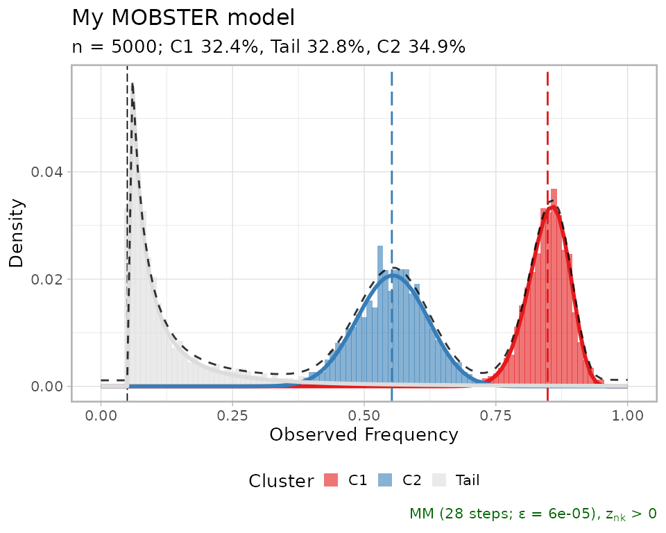

A comparative plot between the fit and data is assembled using cowplot.

cowplot::plot_grid(
  dataset$plot, 
  plot(fit$best), 
  ncol = 2,
  align = 'h')

Giulio Caravagna

21 November, 2025

Input data for `mobster`

Driver annotations

Generating random models and data

Fitting a dataset

Basic plots of a fit

1. Introduction

Giulio Caravagna

21 November, 2025

Input data for mobster

Driver annotations

Generating random models and data

Fitting a dataset

Basic plots of a fit

Input data for `mobster`