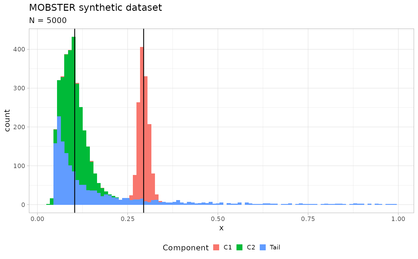
Generate a random MOBSTER model and data.

Generate a random MOBSTER model, its data and creates a plot for it.

Usage

random_dataset(
  N = 5000,
  K_betas = 2,
  pi_tail_bounds = c(0.2, 0.4),
  pi_min = 0.1,
  Betas_separation = 0.1,
  Beta_variance_scaling = 1000,
  Beta_bounds = c(0.1, 0.9),
  shape_bounds = c(1, 1, 3),
  scale = 0.05,
  seed = NULL
)

Arguments

N

Number of samples to generate (mutations).

K_betas

Number of Beta components (subclones).

pi_tail_bounds

2D vector with min and max size of the tail's mutations (proportions).

pi_min

Minimum mixing proportion for every component.

Betas_separation

Minimum separation between the means of the Beta components.

Beta_variance_scaling

The variance of the Beta is generated as U[0,1] and scaled by this value. Values on the order of 1000 give low variance, 100 represents a dataset with quite some dispersion ( compared to a putative Binomial generative model).

Beta_bounds

Range of values to sample the Beta means.

shape_bounds

Range of values to sample the tail shape, default [1, 3],

scale

Tail scale, default 0.05.

seed

The seed to fix the process, default is 123.

Value

A list with the dataset in a tibble, the model parameters and a plot the data.

Examples

x = random_dataset()
print(x)
#> $data
#> # A tibble: 5,000 × 2
#>      VAF simulated_cluster
#>    <dbl> <chr>            
#>  1 0.694 C1               
#>  2 0.726 C1               
#>  3 0.731 C1               
#>  4 0.741 C1               
#>  5 0.769 C1               
#>  6 0.736 C1               
#>  7 0.737 C1               
#>  8 0.748 C1               
#>  9 0.749 C1               
#> 10 0.731 C1               
#> # ℹ 4,990 more rows
#> 
#> $model
#> $model$a
#>       C1       C2 
#> 299.9128 180.8119 
#> 
#> $model$b
#>        C1        C2 
#> 106.60420  30.50675 
#> 
#> $model$shape
#> [1] 1
#> 
#> $model$scale
#> [1] 0.05
#> 
#> $model$pi
#>      Tail        C1        C2 
#> 0.2421595 0.5493651 0.2084753 
#> 
#> 
#> $plot

#>