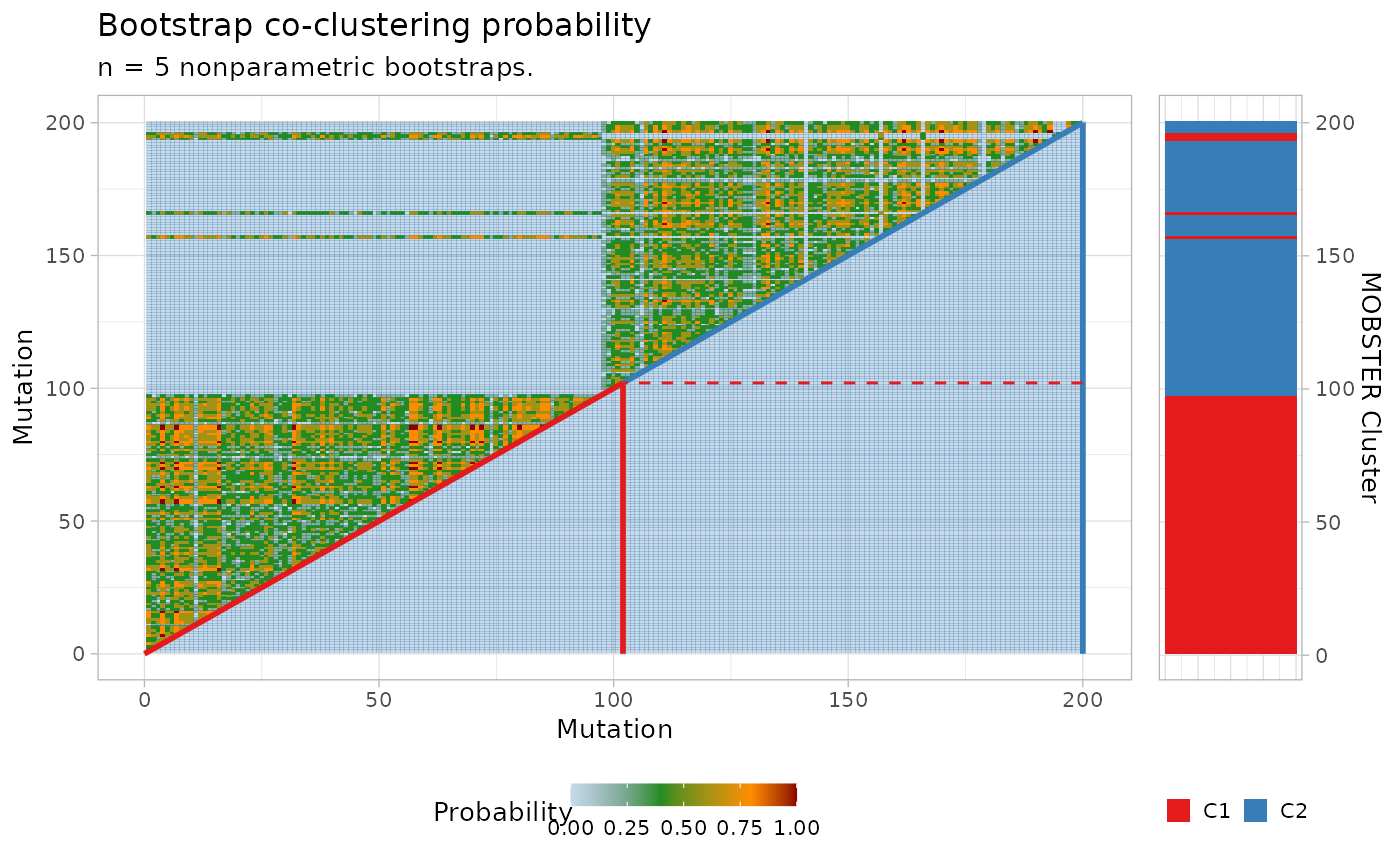
Plot the boostrapped co-clustering probability. — plot_bootstrap

From the results of a call to mobster_boostrap, and the results of a call to bootstrapped_statistics, a figure (heatmap-style) for the boostrapped co-clustering probability is produced assembling plots with cowplot::plot_grid.

Usage

plot_bootstrap_coclustering(
  x,
  bootstrap_results,
  bootstrap_statistics,
  colors = c(Tail = "gainsboro")
)

Arguments

x: A MOBSTER fit.
bootstrap_results: Results of a call to mobster_boostrap.
colors: If provided, these colours will be used for each cluster. If a subset of colours is provided, palette Set1 from RColorBrewer is used. By default the tail colour is provided as 'gainsboro'.
bootstrap_statisticsResults: of a call to bootstrapped_statistics.

Value

A cowplot figure of the bootstrapped co-clustering probability.

Examples

# Random small dataset
dataset = random_dataset(N = 200, seed = 123, Beta_variance_scaling = 100)
x = mobster_fit(dataset$data, auto_setup = 'FAST')
#>  [ MOBSTER fit ] 
#> 
#> ✔ Loaded input data, n = 200.
#> ❯ n = 200. Mixture with k = 1,2 Beta(s). Pareto tail: TRUE and FALSE. Output
#> clusters with π > 0.02 and n > 10.
#> ! mobster automatic setup FAST for the analysis.
#> ❯ Scoring (without parallel) 2 x 2 x 2 = 8 models by reICL.
#> 
#> [easypar] 2025-11-21 08:52:11.229506 - Overriding parallel execution setup [FALSE] with global option : FALSE
#> 
#> 
#> ℹ MOBSTER fits completed in 3.4s.
#> 
#> ── [ MOBSTER ] My MOBSTER model n = 200 with k = 2 Beta(s) without tail ────────
#> ● Clusters: π = 52% [C1] and 48% [C2], with π > 0.
#> ✖ No tail fit.
#> 
#> ● Beta C1 [n = 102, 52%] with mean = 0.58.
#> ● Beta C2 [n = 98, 48%] with mean = 0.11.
#> ℹ Score(s): NLL = -108.12; ICL = -182.58 (-182.58), H = 1.88 (1.88). Fit
#> converged by MM in 70 steps.

# Just 5 resamples of a nonparametric bootstrap run, disabling the parallel engine
options(easypar.parallel = FALSE)
boot_results = mobster_bootstrap(x$best, n.resamples = 5, auto_setup = 'FAST')
#>  [ MOBSTER bootstrap ~ 5 resamples from nonparametric bootstrap ] 
#> 
#> ── [ MOBSTER ] My MOBSTER model n = 200 with k = 2 Beta(s) without tail ────────
#> ● Clusters: π = 52% [C1] and 48% [C2], with π > 0.
#> ✖ No tail fit.
#> 
#> ● Beta C1 [n = 102, 52%] with mean = 0.58.
#> ● Beta C2 [n = 98, 48%] with mean = 0.11.
#> ℹ Score(s): NLL = -108.12; ICL = -182.58 (-182.58), H = 1.88 (1.88). Fit
#> converged by MM in 70 steps.
#> 
#> ℹ Creating nonparametric bootstrap resamples
#> ✔ Creating nonparametric bootstrap resamples ... done
#> 
#> 
#> ── Running fits ─────────────────────────────────── Might take some time ...  ──
#> [easypar] 2025-11-21 08:52:14.716101 - Overriding parallel execution setup [TRUE] with global option : FALSE
#>  [ MOBSTER fit ] 
#> 
#> ✔ Loaded input data, n = 200.
#> ❯ n = 200. Mixture with k = 1,2 Beta(s). Pareto tail: TRUE and FALSE. Output
#> clusters with π > 0.02 and n > 10.
#> ! mobster automatic setup FAST for the analysis.
#> ❯ Scoring (without parallel) 2 x 2 x 2 = 8 models by reICL.
#> 
#> [easypar] 2025-11-21 08:52:14.761779 - Overriding parallel execution setup [FALSE] with global option : FALSE
#> 
#> 
#> ℹ MOBSTER fits completed in 3.8s.
#> 
#> ── [ MOBSTER ] My MOBSTER model n = 200 with k = 2 Beta(s) without tail ────────
#> ● Clusters: π = 50% [C1] and 50% [C2], with π > 0.
#> ✖ No tail fit.
#> 
#> ● Beta C1 [n = 98, 50%] with mean = 0.59.
#> ● Beta C2 [n = 102, 50%] with mean = 0.11.
#> ℹ Score(s): NLL = -101.04; ICL = -168.07 (-168.07), H = 2.23 (2.23). Fit
#> interrupted by MM in 100 steps.
#>  [ MOBSTER fit ] 
#> 
#> ✔ Loaded input data, n = 200.
#> ❯ n = 200. Mixture with k = 1,2 Beta(s). Pareto tail: TRUE and FALSE. Output
#> clusters with π > 0.02 and n > 10.
#> ! mobster automatic setup FAST for the analysis.
#> ❯ Scoring (without parallel) 2 x 2 x 2 = 8 models by reICL.
#> 
#> [easypar] 2025-11-21 08:52:18.668438 - Overriding parallel execution setup [FALSE] with global option : FALSE
#> 
#> 
#> ℹ MOBSTER fits completed in 3.3s.
#> 
#> ── [ MOBSTER ] My MOBSTER model n = 200 with k = 2 Beta(s) without tail ────────
#> ● Clusters: π = 51% [C1] and 49% [C2], with π > 0.
#> ✖ No tail fit.
#> 
#> ● Beta C1 [n = 101, 51%] with mean = 0.59.
#> ● Beta C2 [n = 99, 49%] with mean = 0.11.
#> ℹ Score(s): NLL = -115.21; ICL = -197.42 (-197.42), H = 1.21 (1.21). Fit
#> converged by MM in 62 steps.
#>  [ MOBSTER fit ] 
#> 
#> ✔ Loaded input data, n = 200.
#> ❯ n = 200. Mixture with k = 1,2 Beta(s). Pareto tail: TRUE and FALSE. Output
#> clusters with π > 0.02 and n > 10.
#> ! mobster automatic setup FAST for the analysis.
#> ❯ Scoring (without parallel) 2 x 2 x 2 = 8 models by reICL.
#> 
#> [easypar] 2025-11-21 08:52:22.005144 - Overriding parallel execution setup [FALSE] with global option : FALSE
#> 
#> 
#> ℹ MOBSTER fits completed in 3.3s.
#> 
#> ── [ MOBSTER ] My MOBSTER model n = 200 with k = 2 Beta(s) without tail ────────
#> ● Clusters: π = 50% [C2] and 50% [C1], with π > 0.
#> ✖ No tail fit.
#> 
#> ● Beta C1 [n = 99, 50%] with mean = 0.59.
#> ● Beta C2 [n = 101, 50%] with mean = 0.12.
#> ℹ Score(s): NLL = -108.28; ICL = -182.9 (-182.9), H = 1.87 (1.87). Fit
#> converged by MM in 70 steps.
#>  [ MOBSTER fit ] 
#> 
#> ✔ Loaded input data, n = 200.
#> ❯ n = 200. Mixture with k = 1,2 Beta(s). Pareto tail: TRUE and FALSE. Output
#> clusters with π > 0.02 and n > 10.
#> ! mobster automatic setup FAST for the analysis.
#> ❯ Scoring (without parallel) 2 x 2 x 2 = 8 models by reICL.
#> 
#> [easypar] 2025-11-21 08:52:25.44167 - Overriding parallel execution setup [FALSE] with global option : FALSE
#> 
#> 
#> ℹ MOBSTER fits completed in 3.6s.
#> 
#> ── [ MOBSTER ] My MOBSTER model n = 200 with k = 2 Beta(s) without tail ────────
#> ● Clusters: π = 57% [C1] and 43% [C2], with π > 0.
#> ✖ No tail fit.
#> 
#> ● Beta C1 [n = 113, 57%] with mean = 0.59.
#> ● Beta C2 [n = 87, 43%] with mean = 0.11.
#> ℹ Score(s): NLL = -115.77; ICL = -199.22 (-199.22), H = 0.52 (0.52). Fit
#> converged by MM in 25 steps.
#>  [ MOBSTER fit ] 
#> 
#> ✔ Loaded input data, n = 200.
#> ❯ n = 200. Mixture with k = 1,2 Beta(s). Pareto tail: TRUE and FALSE. Output
#> clusters with π > 0.02 and n > 10.
#> ! mobster automatic setup FAST for the analysis.
#> ❯ Scoring (without parallel) 2 x 2 x 2 = 8 models by reICL.
#> 
#> [easypar] 2025-11-21 08:52:29.10236 - Overriding parallel execution setup [FALSE] with global option : FALSE
#> 
#> 
#> ℹ MOBSTER fits completed in 3.7s.
#> 
#> ── [ MOBSTER ] My MOBSTER model n = 200 with k = 2 Beta(s) without tail ────────
#> ● Clusters: π = 55% [C1] and 45% [C2], with π > 0.
#> ✖ No tail fit.
#> 
#> ● Beta C1 [n = 109, 55%] with mean = 0.59.
#> ● Beta C2 [n = 91, 45%] with mean = 0.13.
#> ℹ Score(s): NLL = -102.08; ICL = -171.04 (-171.04), H = 1.34 (1.34). Fit
#> converged by MM in 29 steps.

boot_stats = bootstrapped_statistics(x$best, boot_results)
#> 
#> ── Computing model frequency ───────────────────────────────────────────────────
#> # A tibble: 1 × 3
#>   Model              Frequency fit.model
#>   <fct>                  <dbl> <lgl>    
#> 1 K = 2 without tail         1 TRUE     
#> 
#> ── Computing confidence Intervals (CI) for empirical quantiles ─────────────────
#> 
#> Mixing proportions 
#>  # A tibble: 3 × 8
#>   cluster statistics          min lower_quantile higher_quantile   max fit.value
#>   <chr>   <chr>             <dbl>          <dbl>           <dbl> <dbl>     <dbl>
#> 1 C1      Mixing proportion 0.496          0.497           0.563 0.565     0.517
#> 2 C2      Mixing proportion 0.435          0.437           0.503 0.504     0.483
#> 3 Tail    Mixing proportion 0              0               0     0         0    
#> # ℹ 1 more variable: init.value <dbl>
#> 
#> Tail shape/ scale 
#>  # A tibble: 0 × 8
#> # ℹ 8 variables: cluster <chr>, statistics <chr>, min <dbl>,
#> #   lower_quantile <dbl>, higher_quantile <dbl>, max <dbl>, fit.value <dbl>,
#> #   init.value <dbl>
#> 
#> Beta peaks 
#>  # A tibble: 4 × 8
#>   cluster statistics     min lower_quantile higher_quantile     max fit.value
#>   <chr>   <chr>        <dbl>          <dbl>           <dbl>   <dbl>     <dbl>
#> 1 C1      Mean       0.586          0.586           0.592   0.593     0.581  
#> 2 C1      Variance   0.00682        0.00690         0.00880 0.00885   0.00893
#> 3 C2      Mean       0.110          0.110           0.128   0.129     0.112  
#> 4 C2      Variance   0.00301        0.00309         0.00446 0.00449   0.00341
#> # ℹ 1 more variable: init.value <dbl>
#> 
#> ── Computing co-clustering probability for nonparametric bootstrap ─────────────
plot_bootstrap_coclustering(x$best, boot_results, boot_stats)
#> Warning: No shared levels found between `names(values)` of the manual scale and the
#> data's colour values.