Fit on real data

Package Setup

For detailed explanation, please visit the package setup.

library(bascule)
#> ✔ Loading bascule. Support : <https://caravagnalab.github.io/bascule/>

knitr::opts_chunk$set(warning = FALSE, message = FALSE)
configure_environment(envname="bascule-env", use_default=TRUE)
py = reticulate::import("pybascule")

Data

We want to analyze 2,682 breast tumour samples from the GEL, ICGC, and HMF cohorts. For this purpose We load the breast tumor type data object breast_data (for more details visit here) from the bascule package, and retrieve the input data (counts) from it.

The counts object is a list which contains two SBS and DBS matrices (data.frame), both with 2682 rows (representing samples), and 96 columns for SBS context and 78 columns for DBS context (representing mutational contexts). The values of the matrices are number of the mutations for corresponding sample and mutational context. The counts matrix can extracted from bascule fit object using the get_input function in the package.

# load breast fit data from package
data("breast_data")

# extract the bascule fit object for breast tumor type
x = breast_data$x

# retrieve the input data of the breast tumor type
counts = get_input(x, matrix=TRUE, reconstructed=FALSE)

# dimensions of SBS and DBS count matrices
dim(counts[["SBS"]])
#> [1] 2682   96
dim(counts[["DBS"]])
#> [1] 2682   78

# display first 5 rows and first 8 columns of SBS and DBS matrices
head(counts[["SBS"]][, 1:8])
#>                A[C>A]A A[C>A]C A[C>A]G A[C>A]T A[C>G]A A[C>G]C A[C>G]G A[C>G]T
#> GEL-2474917-11     131      81      11      70      71      43      10     106
#> GEL-2516072-11     279     199      32     202      68      56      20      69
#> GEL-2905314-11      54      54      11      38      20      19       9      34
#> GEL-2464811-11      48      36       5      35      17      11       3      21
#> GEL-2142020-11      33      18       7      16       8       3       5      14
#> GEL-2674175-11      49      40       5      31      31      17       4      19
head(counts[["DBS"]][, 1:8])
#>                AC>CA AC>CG AC>CT AC>GA AC>GG AC>GT AC>TA AC>TG
#> GEL-2474917-11     0     0     0     0     0     0     1     0
#> GEL-2516072-11     1     0     0     1     0     0     2     1
#> GEL-2905314-11     0     0     0     0     0     0     0     0
#> GEL-2464811-11     0     0     0     1     0     1     0     0
#> GEL-2142020-11     0     0     0     0     0     0     1     0
#> GEL-2674175-11     0     0     0     0     0     0     0     0

As a reference catalogue for breast cancer, we selected signatures SBS1, SBS2, SBS3, SBS5, SBS13, SBS17, SBS18, SBS31, for SBS context and signatures DBS11, DBS13, and DBS20, for the DBS context.

These signature collections are a subset of the COSMIC_sbs_filt and COSMIC_dbs catalogues.

reference_cat <- list(
  "SBS" = COSMIC_sbs_filt[c("SBS1", "SBS2", "SBS3", "SBS5", "SBS13", "SBS17b", "SBS18", "SBS31"), ], 
  "DBS" = COSMIC_dbs[c("DBS11", "DBS13", "DBS2"), ]
)

Fit the Model

based on prior biological knowledge we expect to see the SBS3 as one of the signatures included in both matrices, but in practice, the SBS3 signature is not present in the output of the model. Here we give higher weights to SBS3 using hyperparameters arguments (visit here for more information), to keep this signature in final output.

alpha_conc <- list("SBS3"=100)

We run the model by executing the fit function from bascule package which performs the non-negative matrix factorization to deconvolute the counts matrix to lower rank matrices.

x_pre_refinement = fit(
  counts=counts,
  k_list=0:25,
  cluster=15,
  reference_cat=reference_cat,
  n_steps=3000, lr=0.005,
  seed_list=c(19,255,18321,331),
  hyperparameters=list("alpha_conc"=alpha_conc),
  store_fits=TRUE,
  py=py, 
  CUDA=TRUE, 
  autoguide=TRUE
  )

x_pre_refinement is the output of the models, which is a bascule object, consisting of a list with three components: input, nmf, and clustering.

input contains all the data used to fit the model,
nmf holds the results of the matrix factorization, and
clustering stores the outcomes of the patient clustering phase.

The analysis identified 19 SBS (12 de novo) and 5 DBS (2 de novo) signatures.

After performing NMF, we obtain a list of de novo signatures, but these may be mixtures of different existing signatures inferred by the model. To address this issue, we aim to eliminate any inferred de novo signatures that can be represented as a linear combination of other signatures. This is done using the refine_denovo_signatures function, applied to the bascule object generated from the fit function in the previous step

x_refined = refine_denovo_signatures(x_pre_refinement)

After a refinement step, one de novo signature from SBS context was removed due to its explainability by other signatures. we identified 18 SBS (11 de novo) and 5 DBS (2 de novo) signatures after refinement.

Patients Re-clustering

After applying the signature refinement step, we may obtain a new set of signatures, requiring us to repeat the patient clustering process. To do this, we use the fit_clustering function from the bascule package on the bascule object generated from the refinement step.

x_cls = fit_clustering(
  x_refined,
  cluster=15,
  seed_list=c(19,255,18321,331),
  hyperparameters=list("alpha_conc"=alpha_conc),
  store_fits=TRUE,
  py=py, 
  CUDA=TRUE, 
  autoguide=TRUE
)

we proceeded with the merging step and the tool detected 14 clusters among the breast cancer samples.

Merging

we use the merge_clusters() function to merge the similar clusters. This function will iteratively merge clusters that result similar in the centroid. The merging will stop as soon as the cosine similarity between all pairs of clusters is below cutoff value.

x_merged <- merge_clusters(x_cls)

As we saw in re-clustering step, the tool detected 14 clusters among the breast cancer samples. We then applied an iterative merging function, resulting in 5 clusters, using a cutoff value of 0.8.

Mapping

Later, with help of convert_dn_names function we map the de novo signatures to known signatures from the COSMIC catalogue and the findings from Degasperi et al. If similarity between the de novo signatures and a signature from known catalogues (COSMIC, Degasperi et al.) is higher than threshold, we substitute the de novo signatures with corresponding known signatures, so we can likely take advantage of their known etiology to analyze our results.

x <- convert_dn_names(
  x_merged, 
  reference_cat = list(
    SBS=COSMIC_sbs_filt, 
    DBS=COSMIC_dbs, 
    DEGASPERI_SBS=Degasperi_SBS, 
    DEGASPERI_DBS=Degasperi_DBS
  ), 
  cutoff = 0.8)

within the SBS context, 6 de novo signatures corresponded to COSMIC signatures SBS7a, SBS17b, SBS26, SBS40a, SBS90, and SBS98. Additionally, one de novo signature aligned with the common signature SBS8, and two signatures matched rare signatures SBS44 and SBS97, both from the Degasperi et al. study. In the DBS context, we mapped two de novo signatures to COSMIC signatures DBS14 and DBS20.

Visualization

The bascule object obtained from the previous steps is ready for visualization step. all the visualization functions take the bascule object as the input.

Fitting Scores

The plot_scores visualize the model selection steps. The plot display the BIC and likelihood scores of NMF run for each k value (number of de novo signatures) for both SBS and DBS context. In the plot, the x axis is related to k values and the y axis is related to scores (BIC and Likelihood). The model selects the k value with lowest BIC score in iterative inference process.

plot_scores(x)
#> Joining with `by = join_by(parname, value_fit, seed, type)`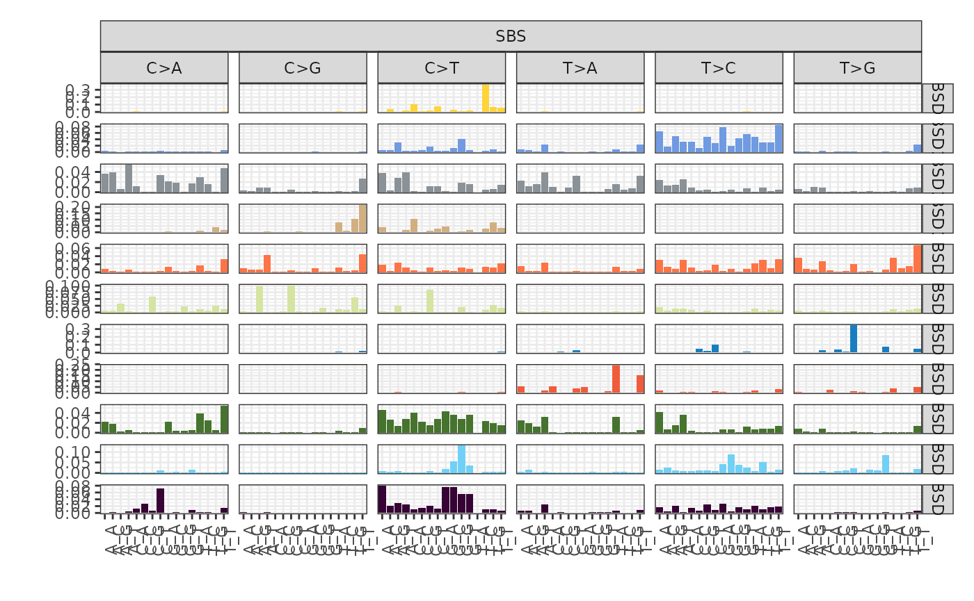

Based on the BIC score, the model with 11 de novo signatures for SBS and 2 de novo signatures for DBS provides the best fit compared to all other models.

Mutational Signatures

We utilize the plot_signatures function to visualize the mutational signatures inferred by the model. The types and signames arguments allow us to specify the context type and the list of signatures to plot. The get_denovo_signames function is used to obtain the list of de novo signature names. Each plot consist of multiple signatures plot with their name on the right hand side.

plot_signatures(x, types = "SBS", signames = get_denovo_signames(x))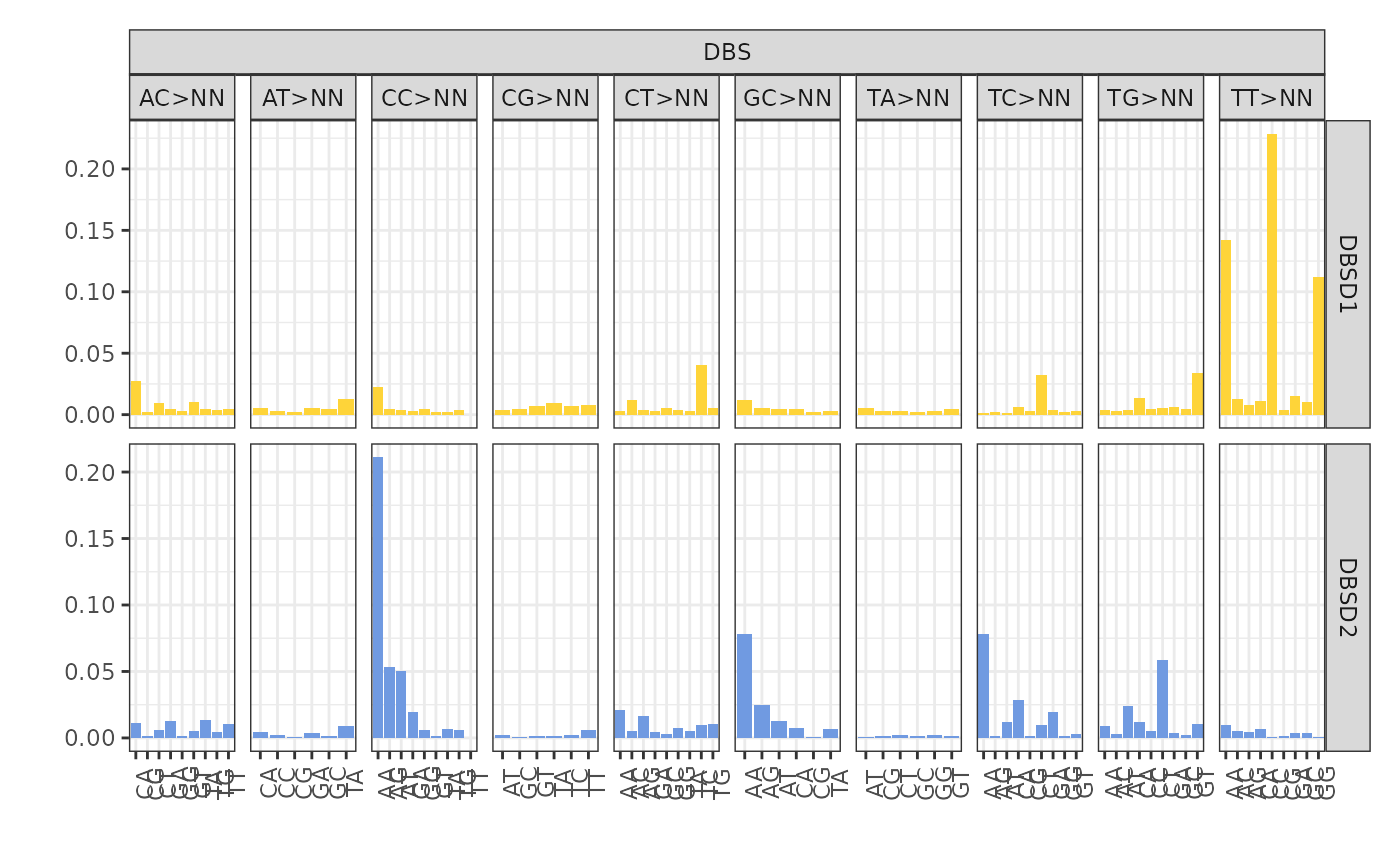

The plot above shows 11 de novo signatures inferred by the tool in SBS context. The x axis shows the 96 possible SBS contexts and the y axis declare their respective density.

plot_signatures(x, types = "DBS", signames = get_denovo_signames(x))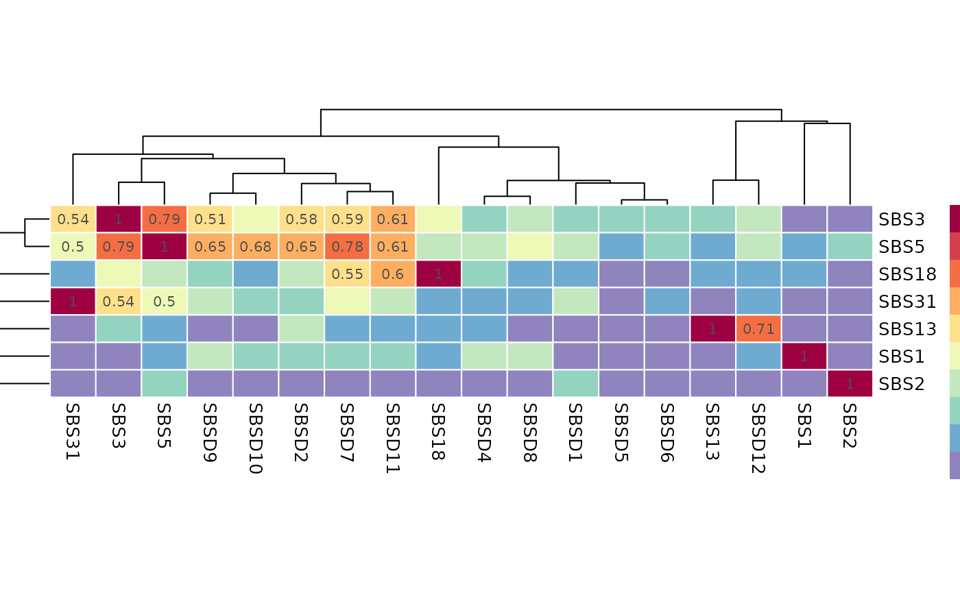

The plot above shows 2 de novo signatures inferred by the tool in DBS context. The x axis shows the 78 possible DBS contexts and the y axis declare their respective density.

Similarity Plot

Function plot_similarity_reference plots the similarity between de novo and COSMIC signatures based on cosine similarity values.

plot_similarity_reference(x)

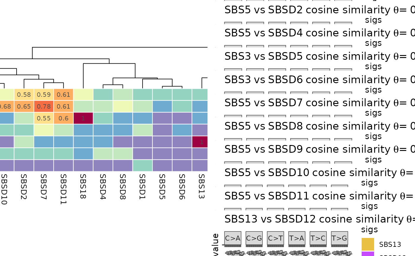
The heatmap plot on the left inspects the similarities between the de novo and COSMIC signatures. The rows are de novo signatures, columns are COSMIC signatures and the values are cosine similarity between the corresponding signatures. On the right you can see the signatures plot comparison of the most similar pairs in the heatmap plot. Since in the mapping step all the de novo signatures were mapped to known signatures with some threshold value (0.8 as default value), here you can see only similarity values below the mentioned threshold in mapping step for de novo signatures.

Clusters Centroids

The plot_centroids() function is used to plot the clustering centroids.

Here, we visualize the clustering centroids of mutational signatures clusters. This plot provides a clear representation of how the mutational signatures are grouped based on their similarities. The plot_centroids function is used to generate this visualization, offering insight into the relationships and distances between different mutational signatures. By examining this plot, we can better understand the patterns and structure of the signature clustering results.

plot_centroids(x)
#> Scale for fill is already present.
#> Adding another scale for fill, which will replace the existing scale.
#> Warning: No shared levels found between `names(values)` of the manual scale and the
#> data's colour values.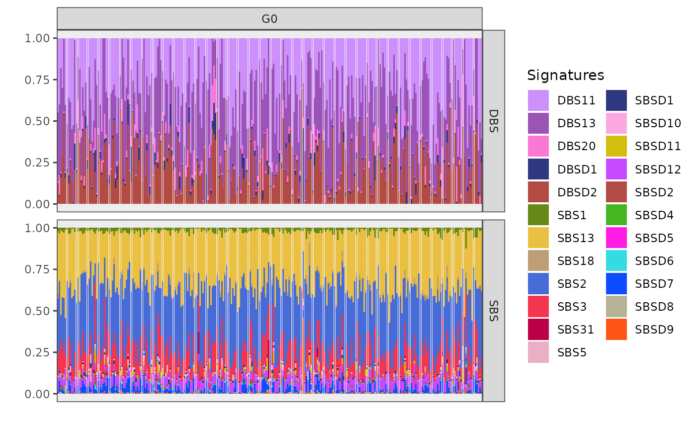

You can inspect the centroids for each cluster in two SBS and DBS context. the x axis defines the clusters, the y axis defines the density of signatures and the colors represent the signatures which are present in the clusters. Using the centroids we can analyze the patients clustering outcome. For detailed information we can follow the exposure plots of each cluster to find out the clustering logic and possible etiology behind it.

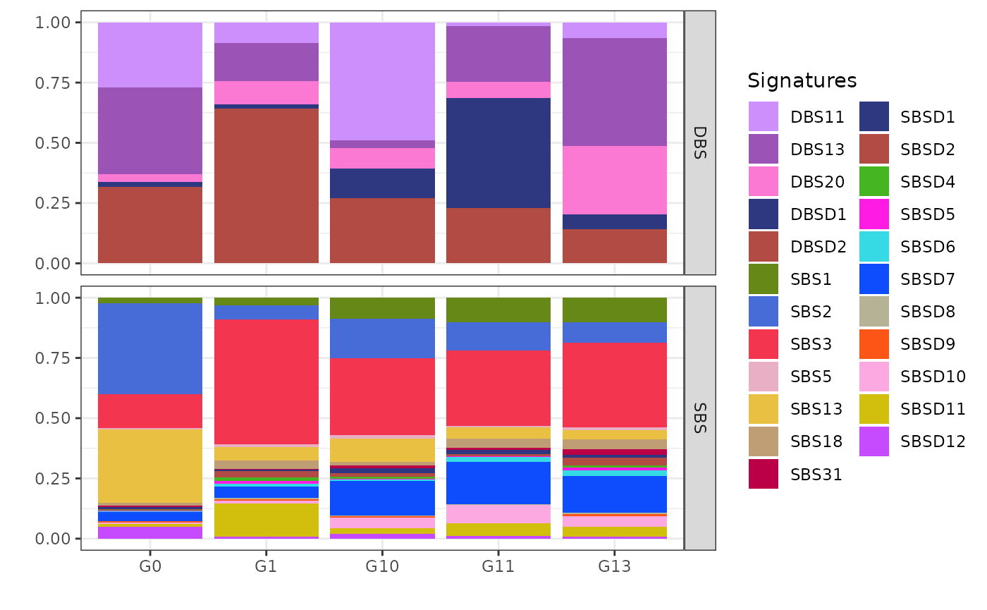
Exposures Matrix

The plot_exposures function is used to visualize the inferred exposure matrix, where x axis represent samples, y axis represents the mutational signatures relative contributions and the colors identify the mutational signatures. The exposure matrix displays the contribution of each mutational signature across different samples. This plot provides a clear overview of how different mutational signatures contribute to the overall mutational profile across the dataset. For clearer visualization, we plot the exposure matrix for each cluster separately. The clusters argument is used to specify which cluster to plot.

plot_exposures(x, clusters = c("G0"))
#> Scale for fill is already present.
#> Adding another scale for fill, which will replace the existing scale.
#> Scale for fill is already present.
#> Adding another scale for fill, which will replace the existing scale.
#> Scale for fill is already present.
#> Adding another scale for fill, which will replace the existing scale.
#> Warning: No shared levels found between `names(values)` of the manual scale and the
#> data's colour values.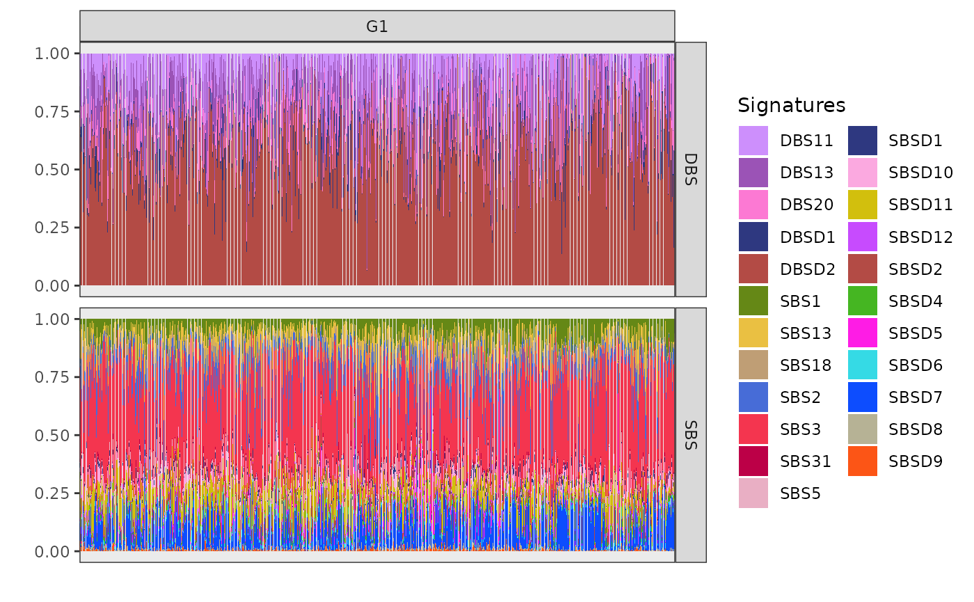

In the exposure plot for cluster G0 (n=272), the dominant mutational signatures are SBS2 and SBS13, along with DBS11, DBS13, and DBSD2 (mapped to DBS2 from COSMIC). These signatures are associated with APOBEC enzyme activity. APOBEC-driven mutational processes are frequently observed in HER2-positive breast cancers, suggesting a strong link between this cluster and HER2-driven tumorigenesis.

plot_exposures(x, clusters = c("G1"))
#> Scale for fill is already present.
#> Adding another scale for fill, which will replace the existing scale.
#> Scale for fill is already present.
#> Adding another scale for fill, which will replace the existing scale.
#> Scale for fill is already present.
#> Adding another scale for fill, which will replace the existing scale.
#> Warning: No shared levels found between `names(values)` of the manual scale and the
#> data's colour values.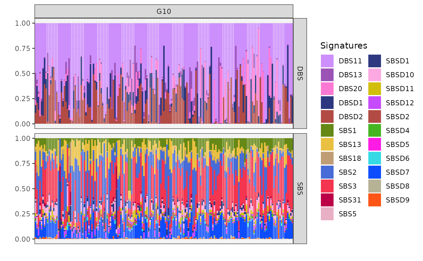

The cluster G1 (n=2058) exposure plot, which is the largest among all, shows a strong presence of SBS3, SBSD11 (mapped to SBS8 from Degasperi et al.), DBSD2 (mapped to DBS2 from COSMIC) and DBS13. SBS3 and DBS13 are caused by homologous recombination deficiency (HRD); DBS2, instead, is linked to smoking in some cancers but is often observed also in cancers not directly linked with tobacco exposure. Based on these prevalent signatures, cluster G1 can be associated with triple-negative breast cancers.

Clusters G10 (n=169), G11 (n=69), and G13 (n=114) share similar SBS patterns, including exposure to SBS1, SBS2, SBS3, SBS11, and SBS13, pointing to a mix of APOBEC activity, HRD, and ageing-related mutational processes. BASCULE can differentiate these three clusters based on DBS exposure.

plot_exposures(x, clusters = c("G10"))
#> Scale for fill is already present.
#> Adding another scale for fill, which will replace the existing scale.
#> Scale for fill is already present.
#> Adding another scale for fill, which will replace the existing scale.
#> Scale for fill is already present.
#> Adding another scale for fill, which will replace the existing scale.
#> Warning: No shared levels found between `names(values)` of the manual scale and the
#> data's colour values.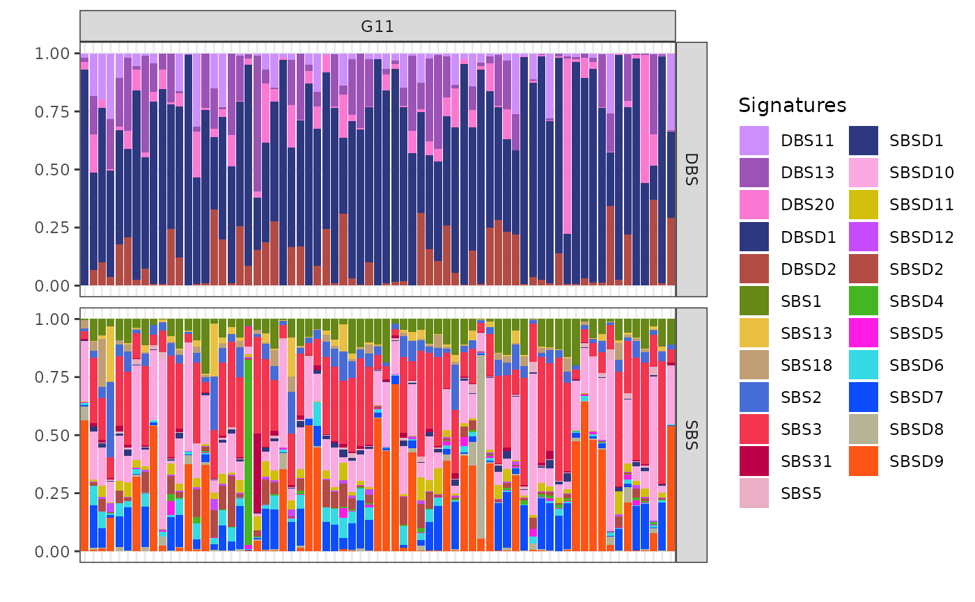

Cluster G10 is notably associated with the mutational signatures DBSD2 (mapped to DBS2 from COSMIC) and DBS11. These signatures are linked to the activity of the APOBEC enzyme family. The strong link between G10 and these signatures suggests that APOBEC activity may be a driving factor behind the mutational processes in this cluster.

plot_exposures(x, clusters = c("G11"))
#> Scale for fill is already present.
#> Adding another scale for fill, which will replace the existing scale.
#> Scale for fill is already present.
#> Adding another scale for fill, which will replace the existing scale.
#> Scale for fill is already present.
#> Adding another scale for fill, which will replace the existing scale.
#> Warning: No shared levels found between `names(values)` of the manual scale and the
#> data's colour values.

The cluster G11 as the smallest cluster is primarily exposed to DBSD1 (mapped to DBS14 from COSMIC), a signature reported as artifactual in COSMIC. However, the presence of DBS13 in G11, suggests that this cluster is also linked to homologous recombination deficiency (HRD).

plot_exposures(x, clusters = c("G13"))
#> Scale for fill is already present.
#> Adding another scale for fill, which will replace the existing scale.
#> Scale for fill is already present.
#> Adding another scale for fill, which will replace the existing scale.
#> Scale for fill is already present.
#> Adding another scale for fill, which will replace the existing scale.
#> Warning: No shared levels found between `names(values)` of the manual scale and the
#> data's colour values.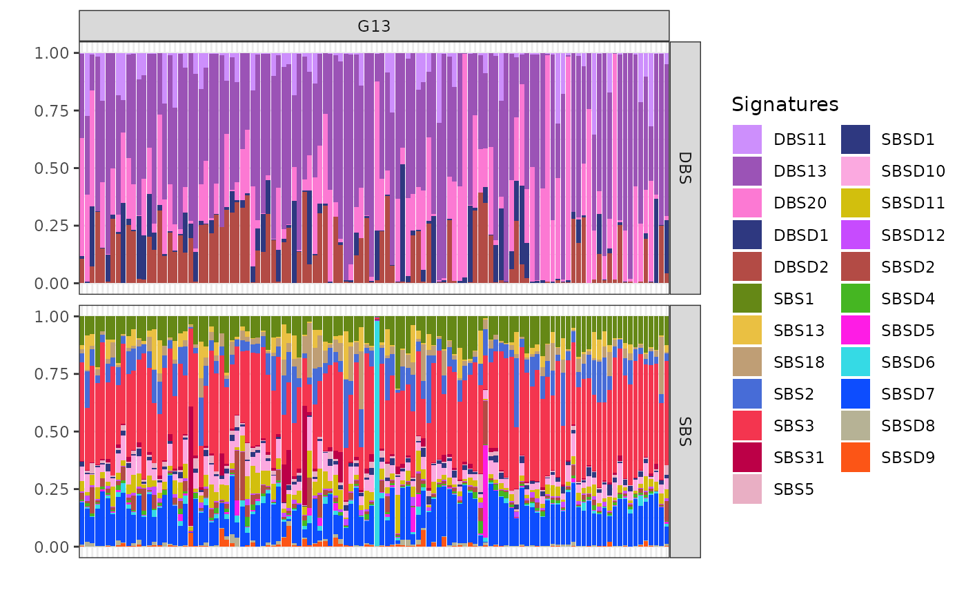

Cluster G13 shows significant exposure to the mutational signatures DBS13 and DBS20. These particular signatures are associated with homologous recombination deficiency (HRD)-related processes. The presence of DBS13 and DBS20 in cluster G13 suggests that the samples in this group may be influenced by similar underlying genomic instability and repair deficiencies.