Inference • bascule

library(bascule)
#> ✔ Loading bascule. Support : <https://caravagnalab.github.io/bascule/>

knitr::opts_chunk$set(warning = FALSE, message = FALSE)
reticulate::install_python(version="3.9.16")
reticulate::py_install(packages="pybascule", 
                       pip=TRUE,
                       python_version="3.9.16")
py = reticulate::import("pybascule")

Load datasets

We can load the data example_dataset, a bascule object containing the true signatures and exposures used to generate the mutation counts matrix. In the object, data for SBS and DBS is reported.

data("synthetic_data")

We can extract the mutation count matrix from the object using the get_input function. With reconstructed=FALSE we are obtaining the observed counts, and not the reconstructed ones computed as the matrix multiplication of exposures and signatures.

counts = synthetic_data$counts
head(counts[["SBS"]][, 1:10])
#>      A[C>A]A A[C>A]C A[C>A]G A[C>A]T A[C>G]A A[C>G]C A[C>G]G A[C>G]T A[C>T]A
#> G1_1     118       7       0      52      10       2       1       5      27
#> G1_2     236      21       5     107      17      12       3      14      67
#> G1_3     132       8       1      50      11       5       1       7      42
#> G1_4     116      15       3      40      10       6       0      12      40
#> G1_5     149      12       3      56      10       3       2      14      49
#> G1_6     161      10       2      66      13       8       4      13      62
#>      A[C>T]C
#> G1_1      10
#> G1_2      35
#> G1_3      19
#> G1_4      26
#> G1_5      16
#> G1_6      25
head(counts[["DBS"]][, 1:10])
#>      AC>CA AC>CG AC>CT AC>GA AC>GG AC>GT AC>TA AC>TG AC>TT AT>CA
#> G1_1     5     1     4     8     4    12     5     0     6    13
#> G1_2     4     1     6     4     3    17     0     1     3    16
#> G1_3     5     0     4     6     1    13     1     0     2    18
#> G1_4     2     0     0     2     0     4     1     1     2     3
#> G1_5     4     0     4     3     0     6     0     1     2     8
#> G1_6     0     0     3     1     0     5     0     1     1     1

We use as reference the COSMIC catalogue for SBS and DBS.

reference_cat = list("SBS"=COSMIC_sbs_filt, "DBS"=COSMIC_dbs)

In the example dataset, the true number of signatures (reference plus de novo) is 5 for both SBS and DBS, thus we can provide as list of K de novo signatures to test values from 0 to 7.

K_list = 0:7

Fit the model

Now, we can fit the model. Let’s first fit the NMF to perform signatures deconvolution.

x = fit(counts=counts, k_list=K_list, n_steps=3000,
        reference_cat=reference_cat,
        keep_sigs=c("SBS1","SBS5"), # force fixed signatures
        store_fits=TRUE, 
        py=py)

x = synthetic_data$x

Visualize the inference scores

You can inspect the model selection procedure. The plot shows for each tested value of K (i.e., number of de novo signatures), the value of the BIC and likelihood of the respective model. In our implementation, the model with lowest BIC is considered as the best model.

plot_scores(x)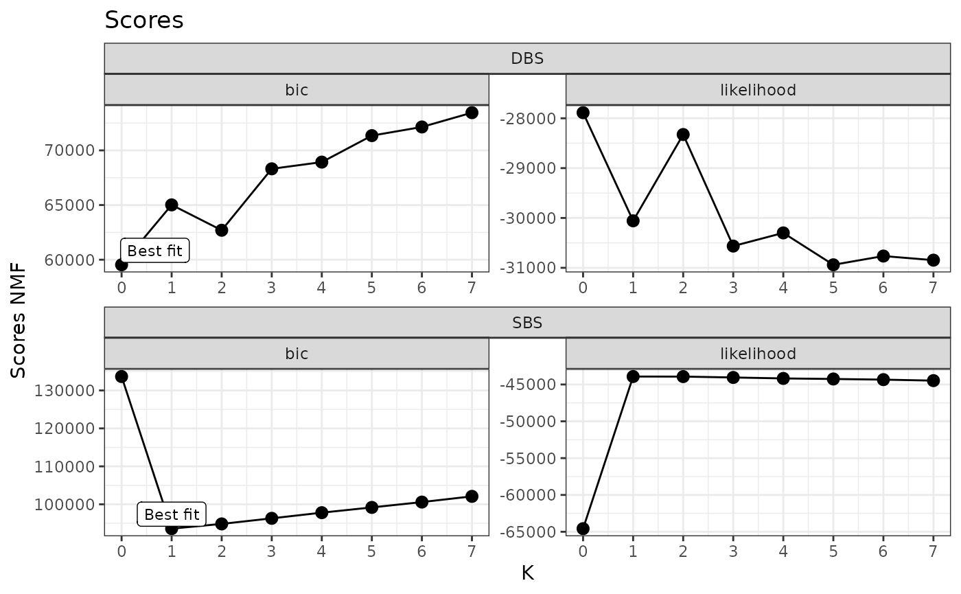

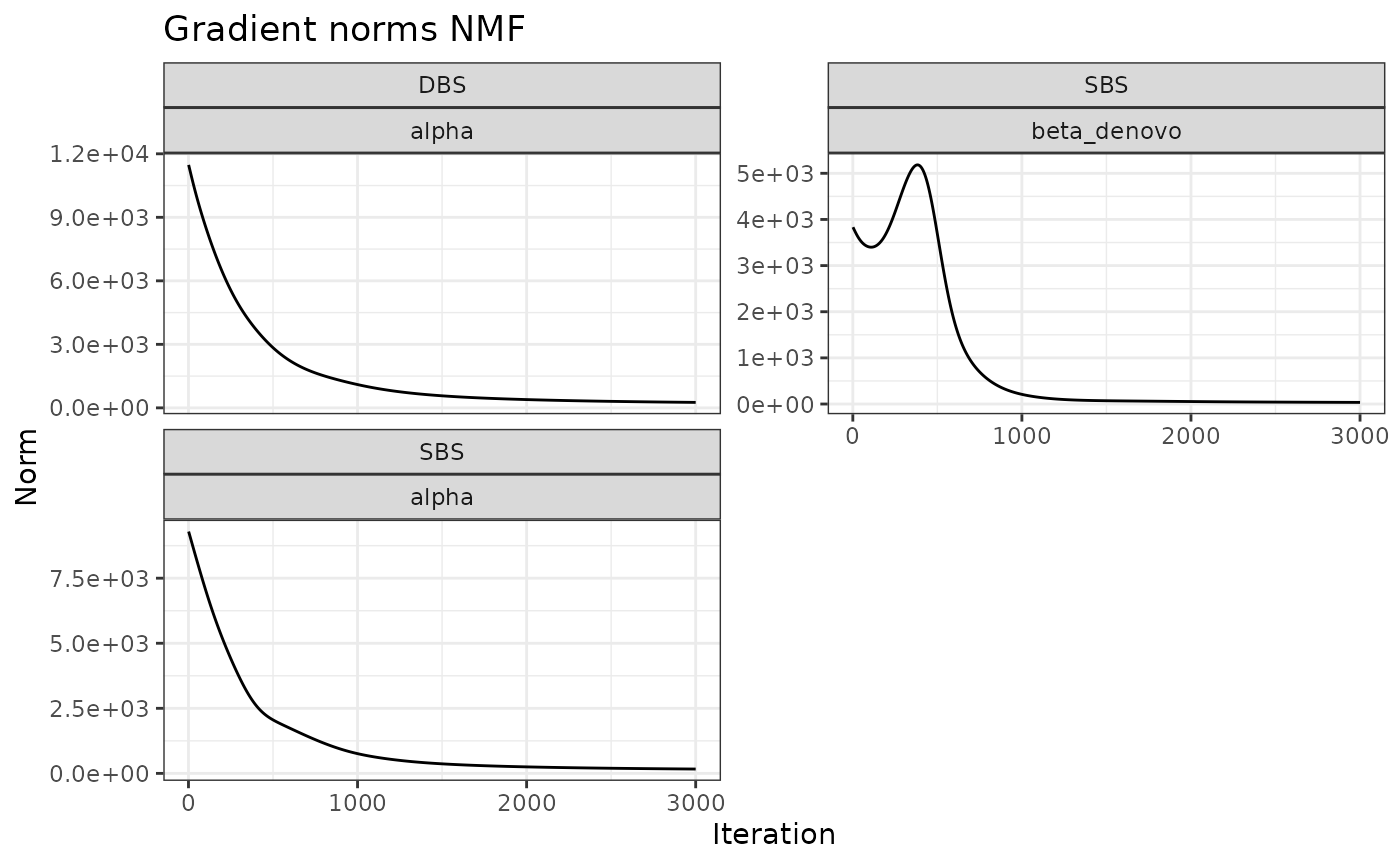
Another variable of interest is the evolution over the iterations of the norms of the gradients for each inferred parameter. A good result, as shown below, is when the norms decreases with inference, reporting an increased stability.

plot_gradient_norms(x)

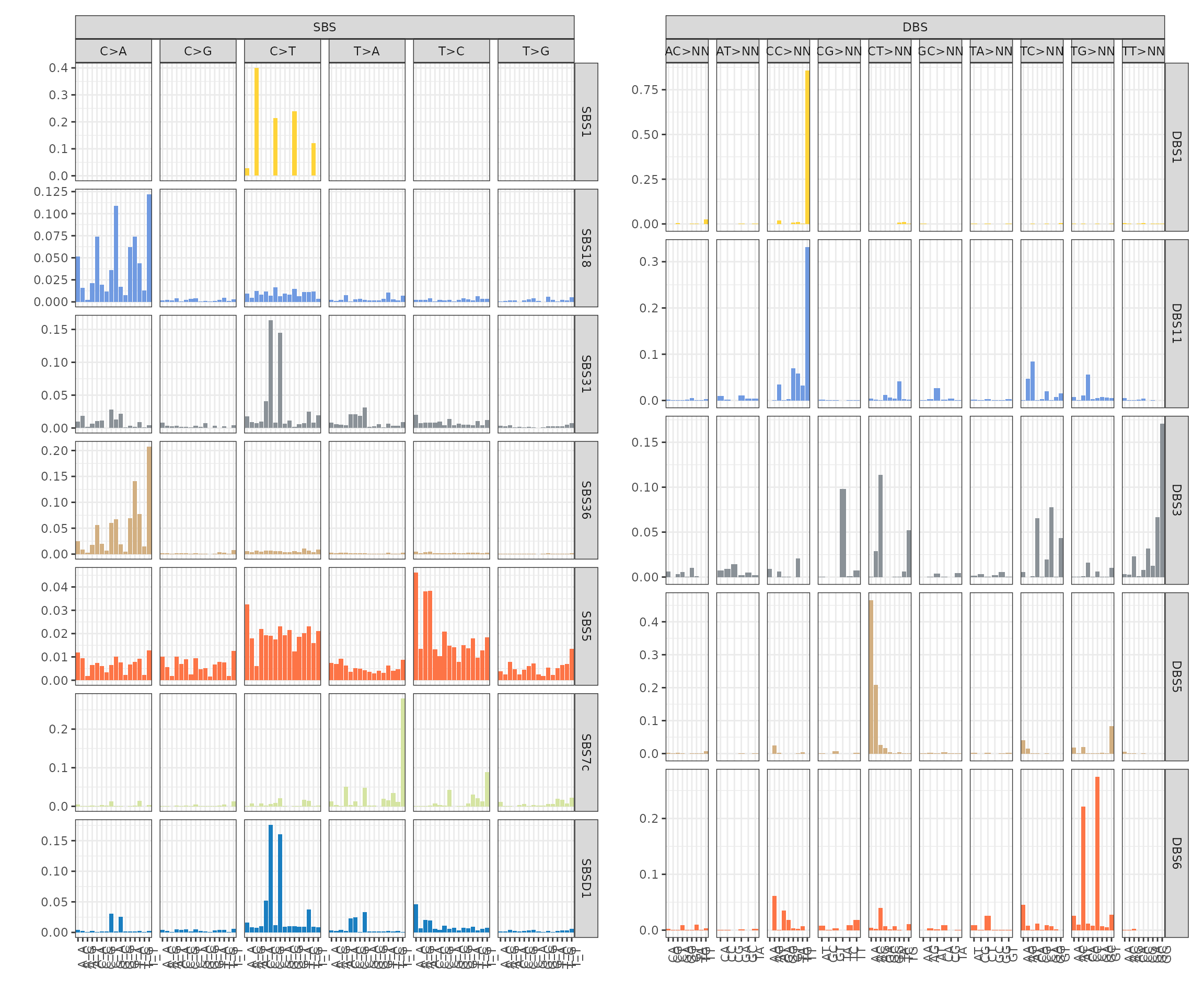
Visualize the inferred parameters

You can visualize the inferred signatures. Here, we notice that from 41 and 20 SBS and DBS signatures, the model only selects 6 and 5 signatures from the catalogue. Moreover, it also infers a denovo signature from the SBS counts.

plot_signatures(x)

Post fit heuristics and clustering

We can notice from the signatures plots a clear similarity between signature SBSD1 and SBS31. We can compute a linear combination on de novo signatures to remove those similar to reference ones. On the refined set of signatures we can run the model to perform clustering of samples based on exposures.

x_refined = refine_denovo_signatures(x)
x_refined_cluster = fit_clustering(x_refined, cluster=3)

x_refined_cluster = synthetic_data$x_refined_cluster

Visualisation of the results

Mutational signatures

The post-fit de novo signatures refinement discarded signature SBSD1, since it showed high similarity with reference signature SBS31.

plot_signatures(x_refined_cluster)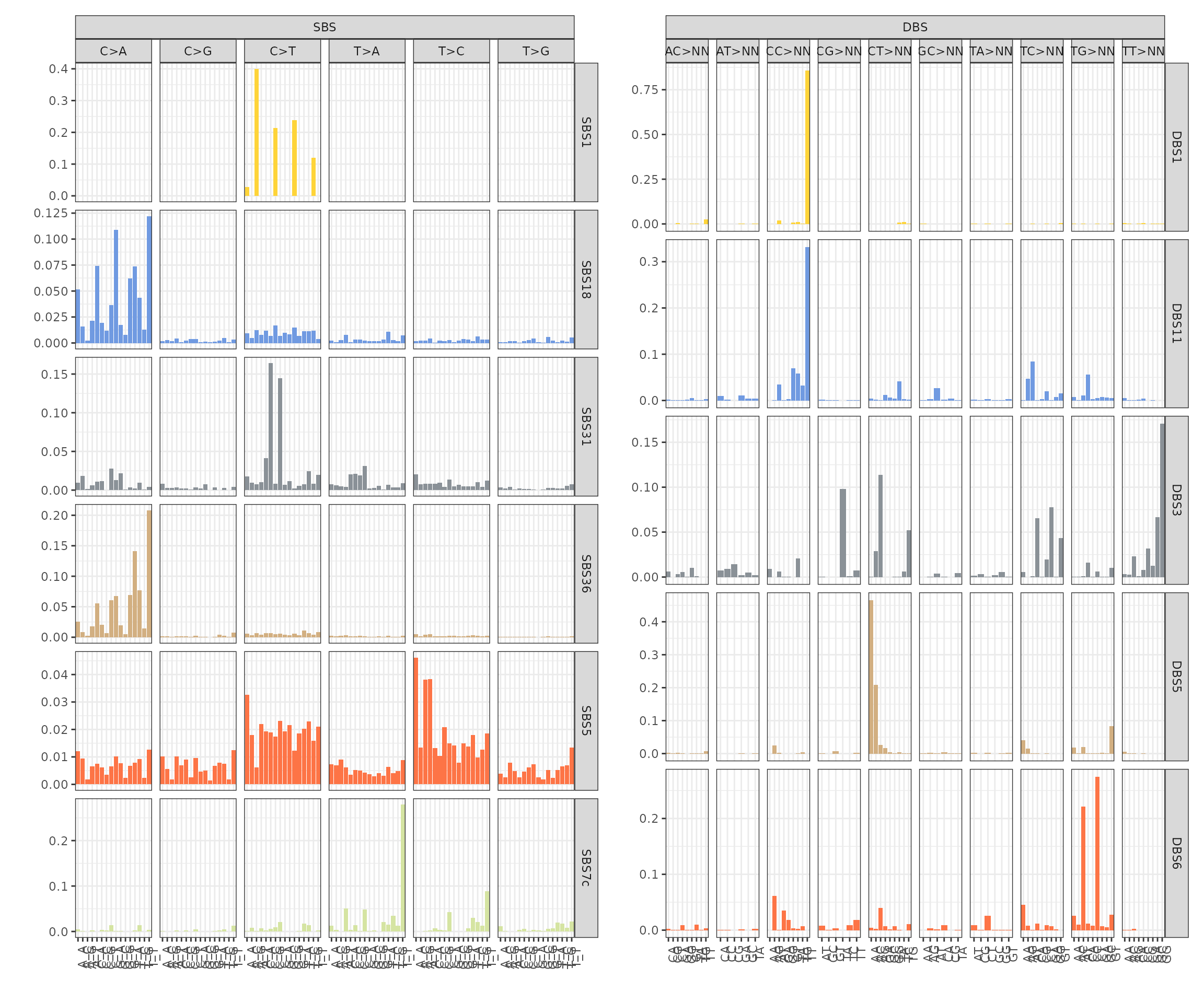

Exposures matrix

We can visualise the exposures for each patient divided by final group assignment. In this case, BASCULE retrieved 3 groups. Each cluster is characterised by a set of SBS and DBS. For instance, group G0 is the largest one and is characterised by signatures DBS1, DBS11 and DBS3, and SBS1, SBS5 and SBS31.

plot_exposures(x_refined_cluster)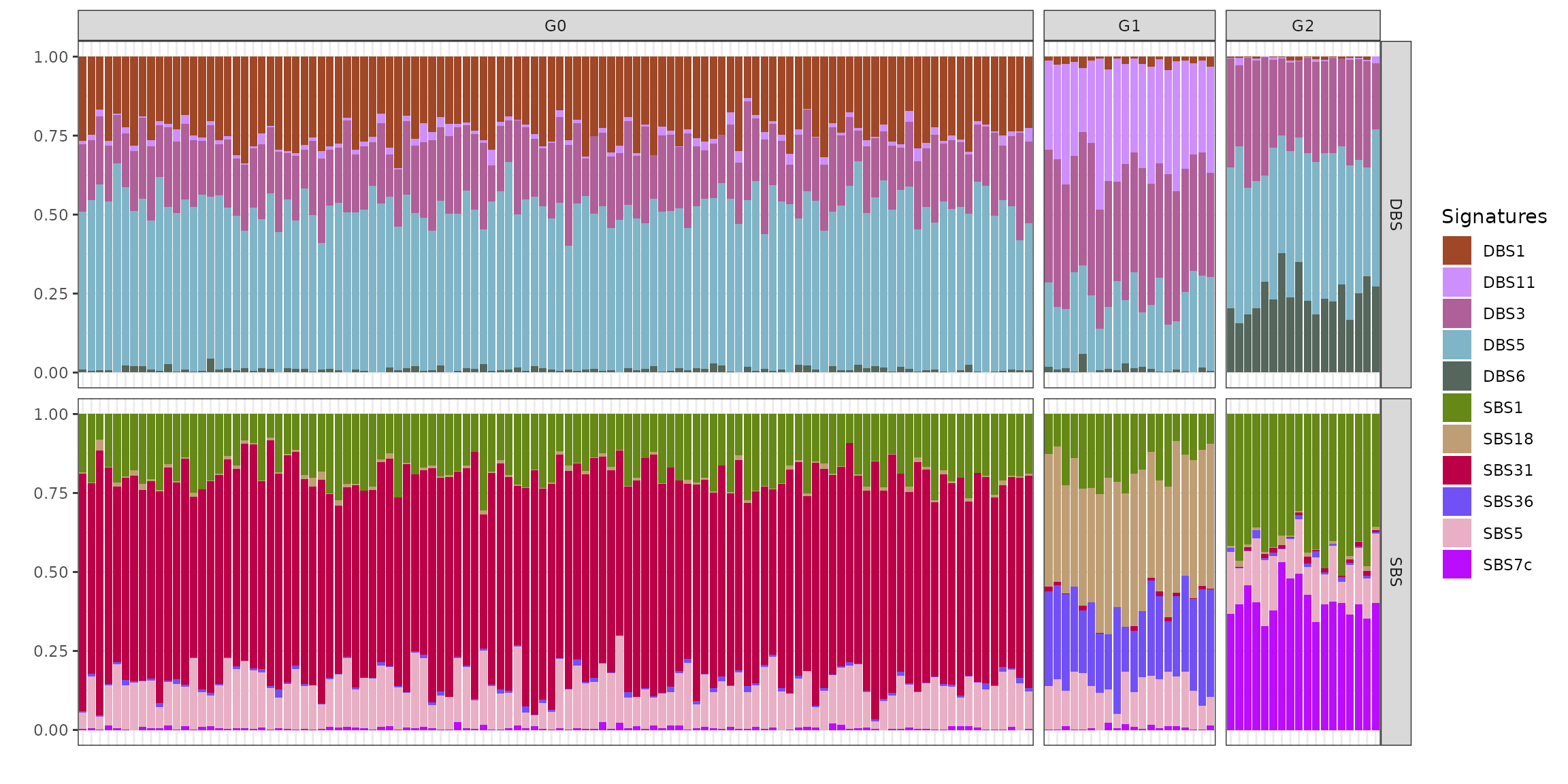

Clustering centroids

We can also inspect the inferred clustering centroids, reporting for each cluster an average of the group-specific signatures exposures.

plot_centroids(x_refined_cluster)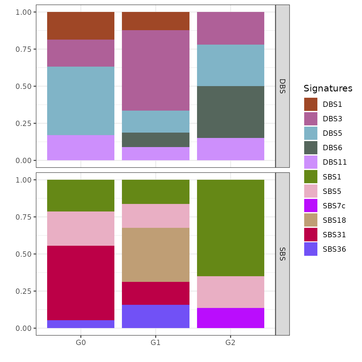

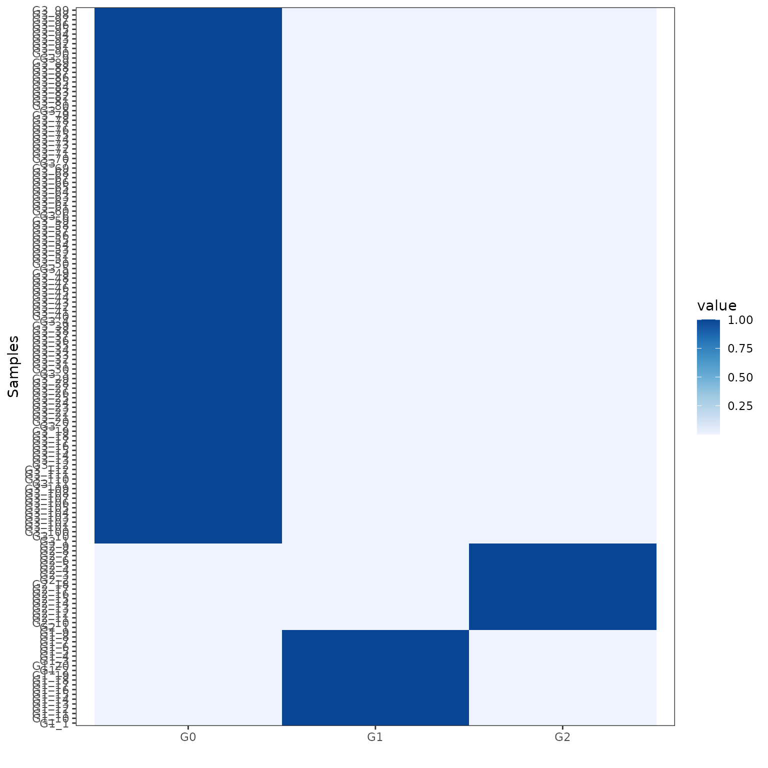
Posterior probabilities

We can finally visualise the posterior probabilities for each sample’s assignment. Each row (samples) of this heatmap sums to 1 and reports the posterior probabilities for each sample to be assigned to each cluster (columns).

plot_posterior_probs(x_refined_cluster)