Disclaimer: RACES/rRACES internally implements the probability distributions using the C++11 random number distribution classes. The standard does not specify their algorithms, and the class implementations are left free for the compiler. Thus, the simulation output depends on the compiler used to compile RACES, and because of that, the results reported in this article may differ from those obtained by the reader.
rRACES/RACES simulate the tumour growth according to two alternative models: the “border”-growth model and the homogeneous-growth model.
The former exclusively admits duplication of cells that have space to duplicate (i.e., cells on the cancer border or near by death cells). The latter allows cell duplications everywhere in the tumour.
The “border”-growth model is the default one. However, users can
switch to the homogeneous growth model by assigning the
SpatialSimulation’s border_growth_model
Boolean field. By setting it to FALSE, the
homogeneous-growth model is used. If, instead, it is set to
TRUE, the simulation evolves according with the
“border”-growth model.
In the remaining part of this article we clarify the differences between the supported growth models by showing that they produce different evolutions of the very same cancer model.
Homogeneous Growth
First of all we need to create a new SpatialSimulation
object and set border_growth_model to
FALSE.
library(rRACES)

set.seed(0)

sim <- SpatialSimulation("Homogeneous Growth")

# Set the homogeneous growth model
sim$border_growth_model <- FALSE

# Set the death activation level to avoid drift
sim$death_activation_level <- 50
Add a mutant A with epigenetic state, let the simulation
evolve until there are 1300 cells of species A+, take two
samples, and let the simulation evolve again for 15 time units.
# Add a mutant
sim$add_mutant(name = "A",
               epigenetic_rates = c("+-" = 0.01, "-+" = 0.01),
               growth_rates = c("+" = 0.1, "-" = 0.08),
               death_rates = c("+" = 0.1, "-" = 0.01))

sim$place_cell("A+", 500, 500)

# Let the simulation evolve until "A+" consists of 1300 cells
sim$run_up_to_size("A+", 1300)
#>  [████████████████████████████████████████] 100% [00m:00s] Saving snapshot

bbox_width <- 15

# Takes two samples
sim$sample_cells("S_1_1",
                 bottom_left = c(480, 480),
                 top_right = c(480 + bbox_width, 480 + bbox_width))

sim$sample_cells("S_1_2",
                 bottom_left = c(500, 500),
                 top_right = c(500 + bbox_width, 500 + bbox_width))

# Let the simulation evolve again for 15 time units
sim$run_up_to_time(sim$get_clock() + 15)
#>  [████████████████████████████████████████] 100% [00m:00s] Saving snapshot
Add a new mutant “B”, let one of the cells in “A” generate a cell in “B”, let the simulation evolve until there are 5000 cells in “B+”, and take again two samples.
sim$add_mutant(name = "B",
               epigenetic_rates = c("+-" = 0.05, "-+" = 0.1),
               growth_rates = c("+" = 0.8, "-" = 0.3),
               death_rates = c("+" = 0.05, "-" = 0.05))

sim$mutate_progeny(sim$choose_cell_in("A"), "B")

sim$run_up_to_size("B+", 5000)
#>  [██████████████████████████--------------] 64% [00m:00s] Cells: 77429 [████████████████████████████████████████] 100% [00m:00s] Saving snapshot

ncells <- 0.9 * bbox_width * bbox_width

bbox <- sim$search_sample(c("B" = ncells), bbox_width, bbox_width)
sim$sample_cells("S_2_1", bbox$lower_corner, bbox$upper_corner)

bbox <- sim$search_sample(c("A" = ncells), bbox_width, bbox_width)
sim$sample_cells("S_2_2", bbox$lower_corner, bbox$upper_corner)
Let us have a look at the simulated tissue and plot the simulation Muller plot.
plot_tissue(sim, num_of_bins = 500)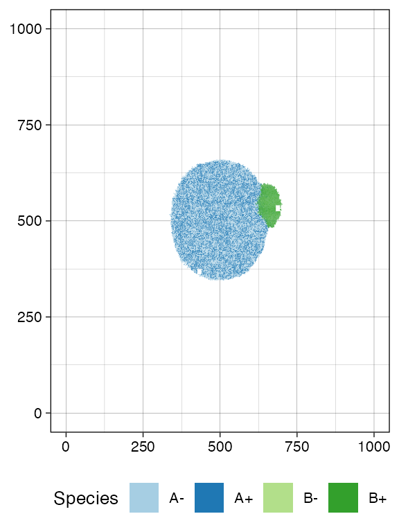
plot_muller(sim)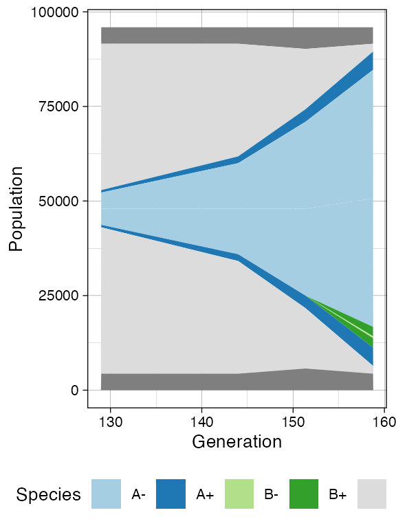
Finally, let us build the ancestor forest of the samples.
library(dplyr)
#>
#> Attaching package: 'dplyr'
#> The following objects are masked from 'package:stats':
#>
#>     filter, lag
#> The following objects are masked from 'package:base':
#>
#>     intersect, setdiff, setequal, union

forest <- sim$get_samples_forest()

plot_forest(forest) %>%
  annotate_forest(forest)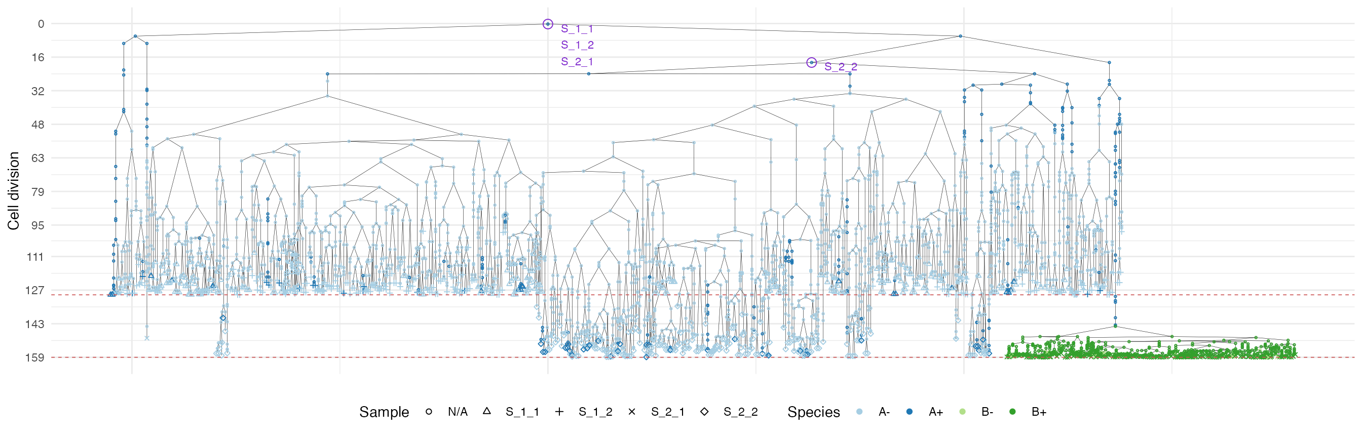
We use a special highlight parameter to add the edges
connecting cells in each sample.
plot_forest(forest, highlight = "S_1_1") %>%
  annotate_forest(forest)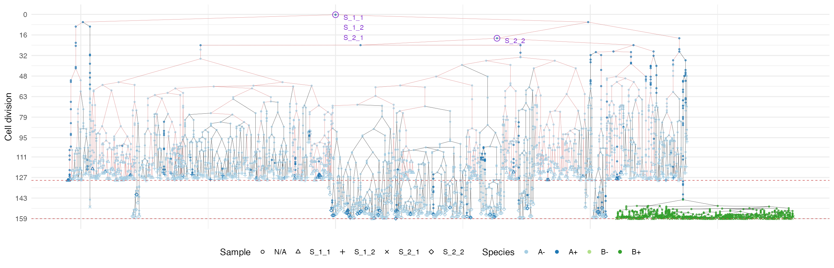
plot_forest(forest, highlight = "S_1_2") %>%
  annotate_forest(forest)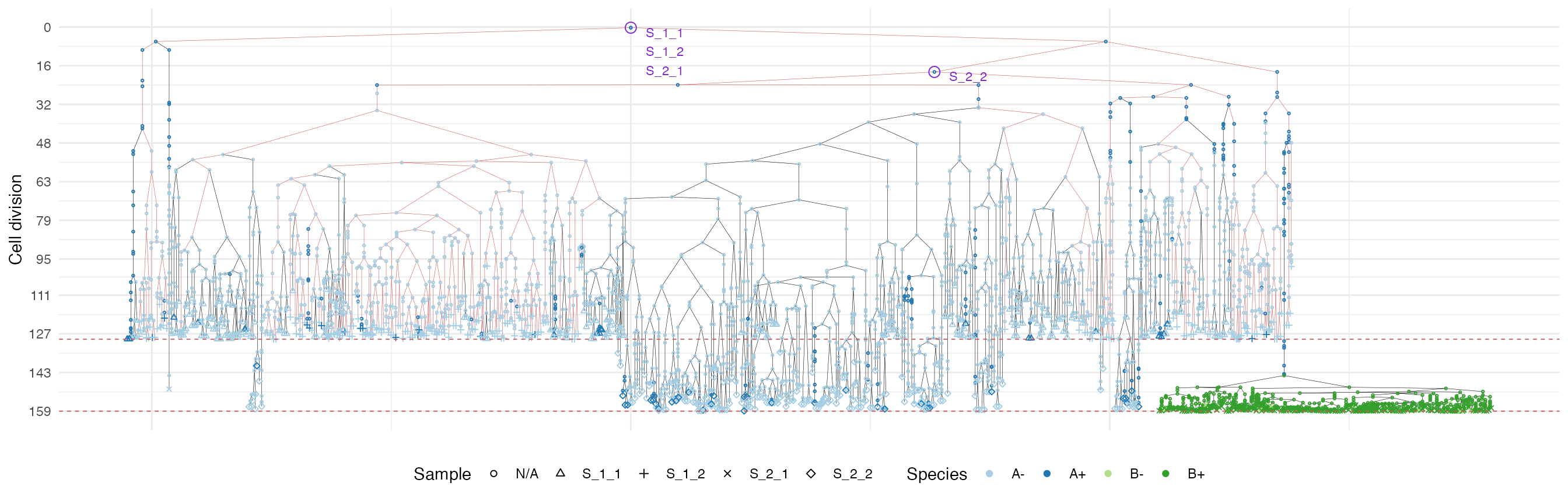
plot_forest(forest, highlight = "S_2_1") %>%
  annotate_forest(forest)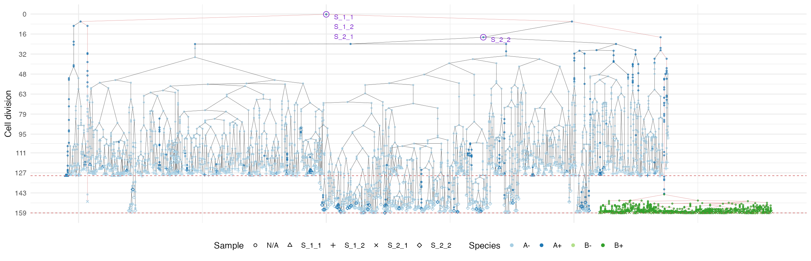
plot_forest(forest, highlight = "S_2_2") %>%
  annotate_forest(forest)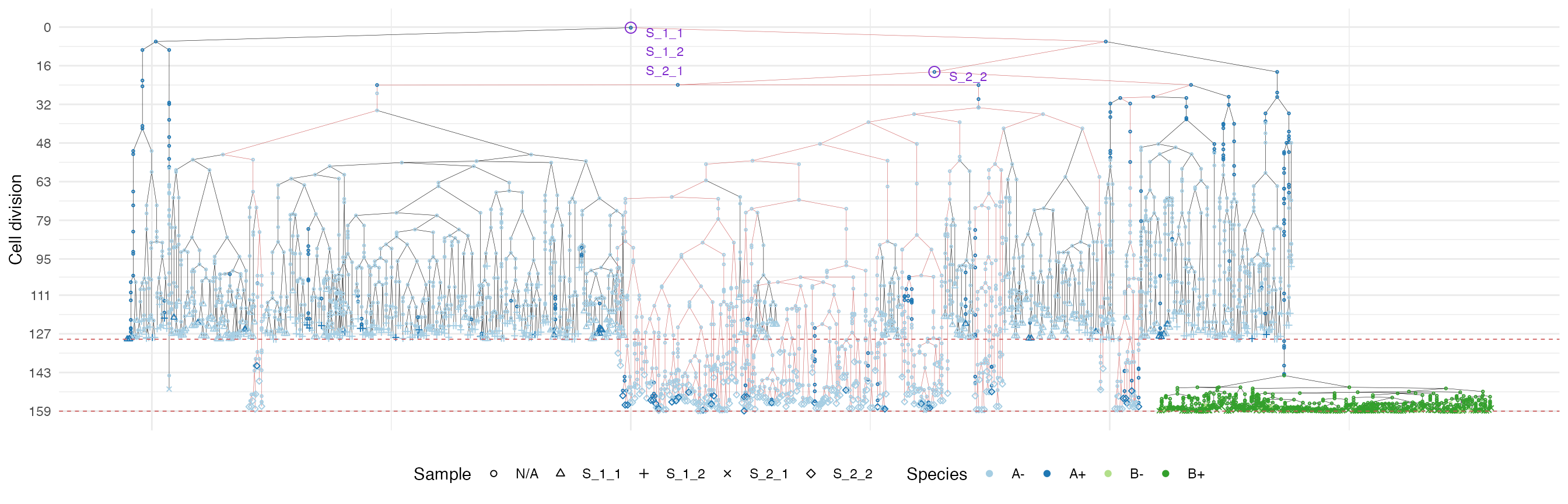
“Border” Growth
We now build a spatial simulation and use the “border” growth model.
set.seed(0)

sim <- SpatialSimulation("Border Growth")

# Setting the "border" growth model is not needed as the
# border growth model is the default.
sim$border_growth_model
#> [1] TRUE

# Set the death activation level to avoid drift
sim$death_activation_level <- 50
Let us repeat what we did in the homogeneous growth model example.
# Add a mutant
sim$add_mutant(name = "A",
               epigenetic_rates = c("+-" = 0.01, "-+" = 0.01),
               growth_rates = c("+" = 0.1, "-" = 0.08),
               death_rates = c("+" = 0.1, "-" = 0.01))

sim$place_cell("A+", 500, 500)

# Let the simulation evolve until "A+" consists of 1300 cells
sim$run_up_to_size("A+", 1300)
#>  [████████████████████████████████--------] 79% [00m:00s] Cells: 28176 [████████████████████████████████████████] 100% [00m:00s] Saving snapshot

bbox_width <- 15

# Takes two samples
sim$sample_cells("S_1_1",
                 bottom_left = c(480, 480),
                 top_right = c(480 + bbox_width, 480 + bbox_width))

sim$sample_cells("S_1_2",
                 bottom_left = c(500, 500),
                 top_right = c(500 + bbox_width, 500 + bbox_width))

# Let the simulation evolve again for 15 time units
sim$run_up_to_time(sim$get_clock() + 15)
#>  [████████████████████████████████████████] 100% [00m:00s] Saving snapshot

# Add a new mutant
sim$add_mutant(name = "B",
               epigenetic_rates = c("+-" = 0.05, "-+" = 0.1),
               growth_rates = c("+" = 0.8, "-" = 0.3),
               death_rates = c("+" = 0.05, "-" = 0.05))


# Let one of the "A" cells generate a cell in "B"
sim$mutate_progeny(sim$choose_cell_in("A"), "B")

# Let the simulation evolve until "B+" consists of 5000 cells
sim$run_up_to_size("B+", 5000)
#>  [███████████████████████-----------------] 55% [00m:00s] Cells: 64653 [████████████████████████████████████████] 100% [00m:00s] Saving snapshot

ncells <- 0.9 * bbox_width * bbox_width

bbox <- sim$search_sample(c("B" = ncells), bbox_width, bbox_width)
sim$sample_cells("S_2_1", bbox$lower_corner, bbox$upper_corner)

bbox <- sim$search_sample(c("A" = ncells), bbox_width, bbox_width)
sim$sample_cells("S_2_2", bbox$lower_corner, bbox$upper_corner)
Let us have a look at the simulated tissue and plot the simulation Muller plot.
plot_tissue(sim, num_of_bins = 500)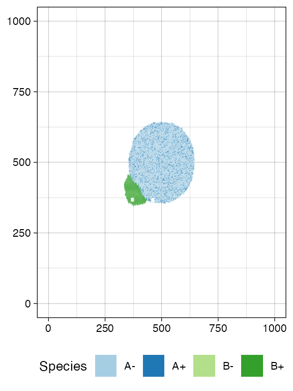
plot_muller(sim)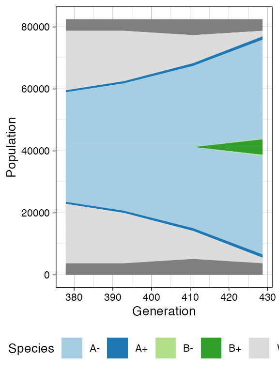
Once more, let us build the ancestor forest of the samples.
forest <- sim$get_samples_forest()

plot_forest(forest) %>%
  annotate_forest(forest)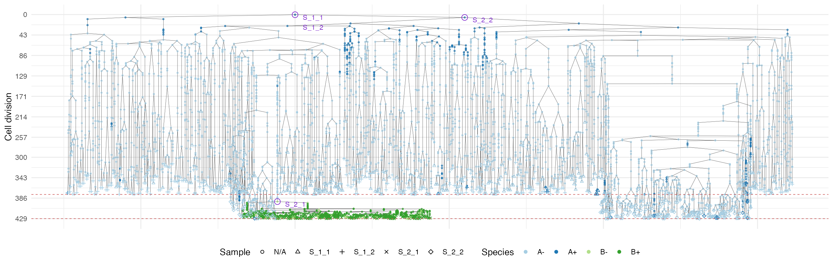
We use a special highlight parameter to add the edges
connecting cells in each sample.
plot_forest(forest, highlight = "S_1_1") %>%
  annotate_forest(forest)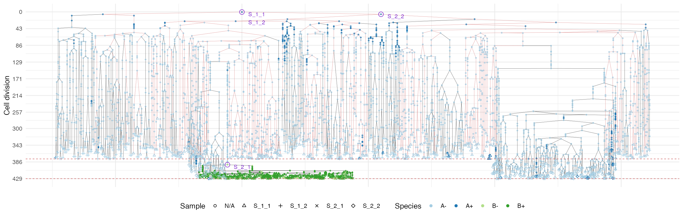
plot_forest(forest, highlight = "S_1_2") %>%
  annotate_forest(forest)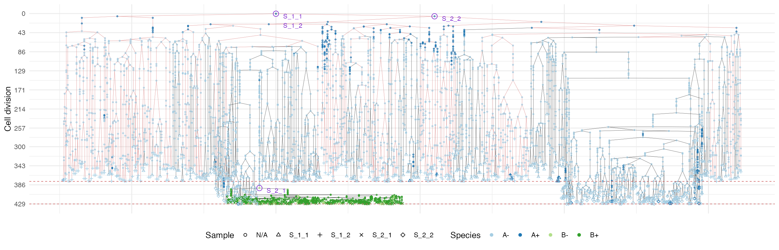
plot_forest(forest, highlight = "S_2_1") %>%
  annotate_forest(forest)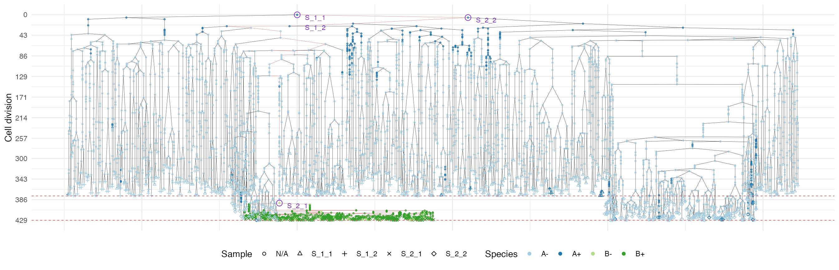
plot_forest(forest, highlight = "S_2_2") %>%
  annotate_forest(forest)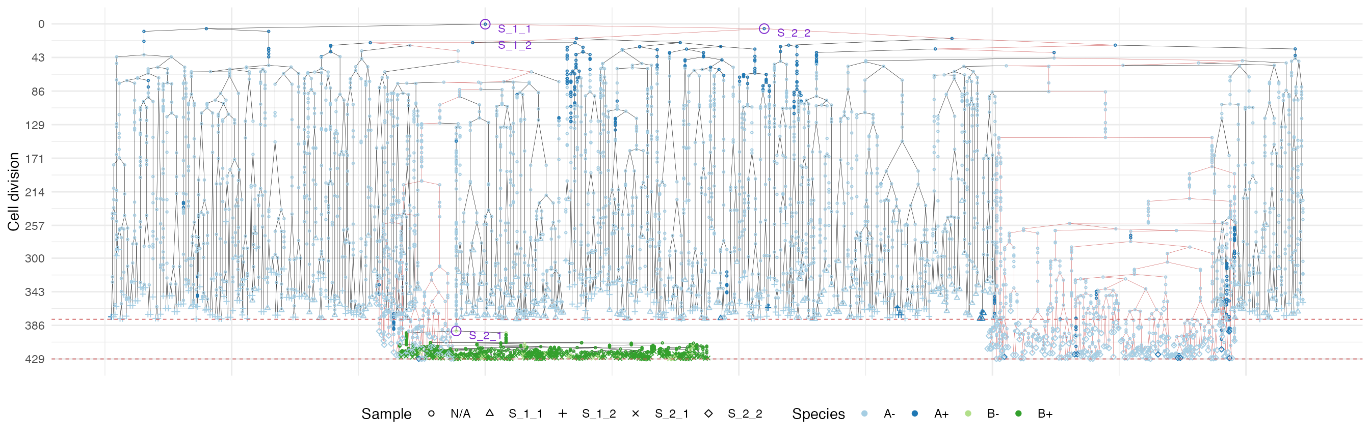
It is easy to see the differences in the analoguous plots of the above examples.
First of all, the cancer growth is slower when subject to the “border”-growth model than when the homogeneous-growth model is used. This is due to the fact that the internal cells cannot duplicate in the former growth model, thus, the number of cells active for duplication is always greater in it, than in the homogeneous-growth model.
Moreover, spatial closeness and closeness in the samples ancestor
forest are strictly related in the “border” growth model, whereas they
appear to be loosely related in the homogeneous growth model. This
features can be easily spotted in the forest plots when the sample
S_2_1 is selected near the external tumour border.