Disclaimer: RACES/rRACES internally implements the probability distributions using the C++11 random number distribution classes. The standard does not specify their algorithms, and the class implementations are left free for the compiler. Thus, the simulation output depends on the compiler used to compile RACES, and because of that, the results reported in this article may differ from those obtained by the reader.
To simulate a tissue the following steps are required:
creation of a tissue;
introduction of cells in the tissue;
actual simulation.
The simulation is managed by an object of the S4 class
SpatialSimulation, wich allows to program the tissue
evolution over time, adding new cells as far as the simulation
progresses. The state of the simulation and tissue can be visualised
using ggplot-powered plots.
Tissue specification
To perform a simulation a new object of class
SpatialSimulation must be created.
library(rRACES)

# Default constructor
sim <- SpatialSimulation()
This automatically builds a 1000x1000-cells tissue - which can host
million cells - and sets the name of the simulation to be
races_<date>_<hour>.
A simulation custom name can be specified as it follows.
library(rRACES)

# set the seed of the random number generator
set.seed(0)

# Call your simulation "Test"
sim <- SpatialSimulation("Test")
The set.seed() call is not mandatory and can be avoided;
however, it is highly suggested to guarantee the simulation
repeatability.
In order to save the simulation progresses in the disk and recover it
in the future, use the optional Boolean parameter
save_snapshots. By setting save_snapshots to
TRUE, the simulation progresses will be saved in a
directory whose name is the name of the simulation.
# The progresses of the simulation will saved in the "Test" folder.
# If the directory "Test" already exists an exception is raised.
sim <- SpatialSimulation("Test", save_snapshots = TRUE)
Class SpatialSimulation exports a
SpatialSimulation$show() method to get information on the
current object.
sim
#> ──  rRACES   D   S   M  Test ──────────────────────────── ▣  [1000x1000]  ⏱ 0 ──
#> ✖ The simulation has no samples yet!
The sim object exposes also methods to get information
about the simulation and control it.
# Get the simulation directory, i.e., "Test"
sim$get_name()
#> [1] "Test"

# Get the tissue size, i.e., c(1000,1000)
sim$get_tissue_size()
#> [1] 1000 1000
Custom Tissue Sizes
The tissue sizes can be specified during simulation creation using
the parameters width and height.
# build a spatial simulation whose tissue has width 1200 and
# height 900
sim <- SpatialSimulation("Test", width=1200, height=900)

# Get the tissue size, i.e., c(1200,900)
sim$get_tissue_size()
#> [1] 1200  900
Species specification
In order to simulate the evolution of some species we need to add
them to sim. This process defines the evolutionary
parameters of the species.
A mutant is a set of cells having the same (potentially unknown) driver mutations. Cells in the same mutant can have different liveness rates due to different epigenetic states.
A species is a mutant with an optional epigenetic state. At
this point in the simulation, the mutant is just a name (A,
B, ..) that, at a later stage could be linked to mutations
of interest. The epigenome is a binary feature of a species that is
represented by epistates +/- (positive and
negative status). This is an abstraction, and could represent an
active/inactive state linked to a promoter methylation or, more broadly,
a phenotype. The evolution of mutants is non-reversible (no-back
mutations model), while the evolution among epistates is potentially
reversible.
For example, if we define two mutants A and
B with their epistates +/-, we
have 4 distinct species: A+ and A-, as well as
B+ and B-.
Hybrid models can be obtained, e.g., a mutant A (with no
epistates), together with B+ and B-.
Evolutionary parameters
We use a notation common in linear birth-death processes. If a
species A has no epistates then its stochastic behaviour is
defined by the state-change rates
where:
- is a growth rate for cells that duplicate;
- is a death rate for cells that duplicate.
Instead, if the species has epistate + (denoted
)
and - (denoted
),
then its stochastic behaviour is defined by the state-change rates
where the rates and are as above, and or are the ratesat which cells of a certain epistate duplicate and flip the epigenetic marker of one of the progeny.
sim$add_mutant(name = "A",
               epigenetic_rates = c("+-" = 0.01, "-+" = 0.01),
               growth_rates = c("+" = 0.2, "-" = 0.08),
               death_rates = c("+" = 0.05, "-" = 0.01))

# updated object (counts refer to number of cells of each species)
sim
#> ──  rRACES   D   S   M  Test ───────────────────────────── ▣  [1200x900]  ⏱ 0 ──
#>
#> ── Species: 2, with epigenetics
#>
#>    =======  ====  ====  ====  ======  ===
#>    species   λ      δ    ε    counts   %
#>    =======  ====  ====  ====  ======  ===
#>         A-  0.08  0.01  0.01    0     NaN
#>         A+  0.20  0.05  0.01    0     NaN
#>    =======  ====  ====  ====  ======  ===
#>
#> ── Firings: 0 total
#> ✖ The simulation has no samples yet!

# Get the simulation species and their rates
sim$get_species()
#>   mutant epistate growth_rate death_rate switch_rate
#> 1      A        -        0.08       0.01        0.01
#> 2      A        +        0.20       0.05        0.01
A mutant without epistates could be added as
# Not run
sim$add_mutant(name = "A", growth_rates = 0.2, death_rates =  0.1)
To be able to simulate the model, an initial cell needs to be displaced in the tissue.
# We add one cell of species A+ (mutant A in epistate +) in
# position (500, 500).
sim$place_cell("A+", 500, 500)
Visualisations
We can query the current state of the simulation, and extract the position of each cell in the tissue.
# Counts per species
sim$get_counts()
#>   mutant epistate counts overall
#> 1      A        -      0       0
#> 2      A        +      1       1

# Cells position (one so far)
sim$get_cells()
#>   cell_id mutant epistate position_x position_y
#> 1       0      A        +        500        500
These information can be plot. Note that the tissue visualisation uses hexagonal bins to avoid rastering delays when the simulation uses thousands of cells.
# Piechar for counts
plot_state(sim)
# Spatial distribution for the whole tissue (hexagonal bins)
plot_tissue(sim)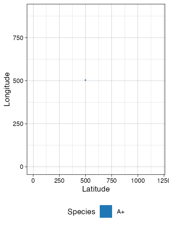
Note: since the plots are done with
ggplotthey can be assembled and customised.
Species Evolution
There are 4 ways to let the simulation evolve:
- advancing until the number of cells in a species reaches a given threshold ;
- advancing until a new time is reached;
- advancing until a desired number of firings (of one particular event) has occurred;
- advancing until a formula is not satisfied by the simulation status
(advanced topic; see
vignette("run_until")).
Size-Based Simulation
We can run the simulation up to when we have
;
cells of species A+
# Counts per species is now 0
sim$get_counts()
#>   mutant epistate counts overall
#> 1      A        -      0       0
#> 2      A        +      1       1

sim$run_up_to_size("A+", 500)
#>  [████████████████████████████████████████] 100% [00m:00s] Saving snapshot

# Counts per species now reports 500 for A+
sim$get_counts()
#>   mutant epistate counts overall
#> 1      A        -     42      70
#> 2      A        +    500    1648

plot_tissue(sim)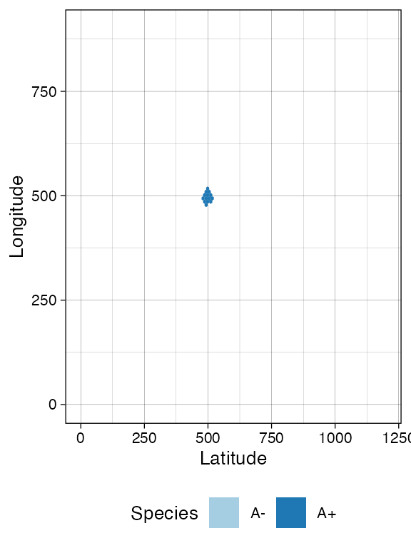
Firing-Based Simulation
The number of times each event has fired is accessible
# Get the number of fired event per species
sim$get_firings()
#>    event mutant epistate fired
#> 1  death      A        -     8
#> 2 growth      A        -    17
#> 3 switch      A        -     3
#> 4  death      A        +   290
#> 5 growth      A        +   822
#> 6 switch      A        +    36
A small number of cell deaths have occurred in species
A- up to this point, so we can simulate the system until
there are 100 of them.
sim$run_up_to_event("death", "A-", 100)
#>  [████████████████████████████████████████] 100% [00m:00s] Saving snapshot

# The row "death", for "A" "-" now reports 100
sim$get_firings()
#>    event mutant epistate fired
#> 1  death      A        -   100
#> 2 growth      A        -   419
#> 3 switch      A        -    51
#> 4  death      A        +  3042
#> 5 growth      A        +  6022
#> 6 switch      A        +   281
# Plot the tissue by using 200 bins
plot_tissue(sim, num_of_bins = 200)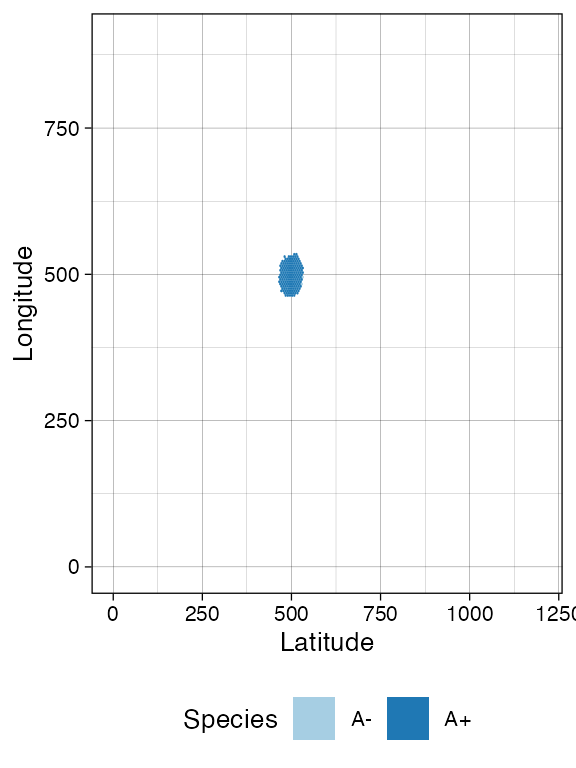
Clock-Based Simulation
It is also possible to take the current simulation clock as reference, and simulate further.
# Get the simulation clock
sim$get_clock()
#> [1] 81.62523

# Run the simulation for other 15 time units
sim$run_up_to_time(sim$get_clock() + 15)
#>  [████████████████████████████████████████] 100% [00m:00s] Saving snapshot

# Get again the simulation clock
sim$get_clock()
#> [1] 96.62686
plot_tissue(sim)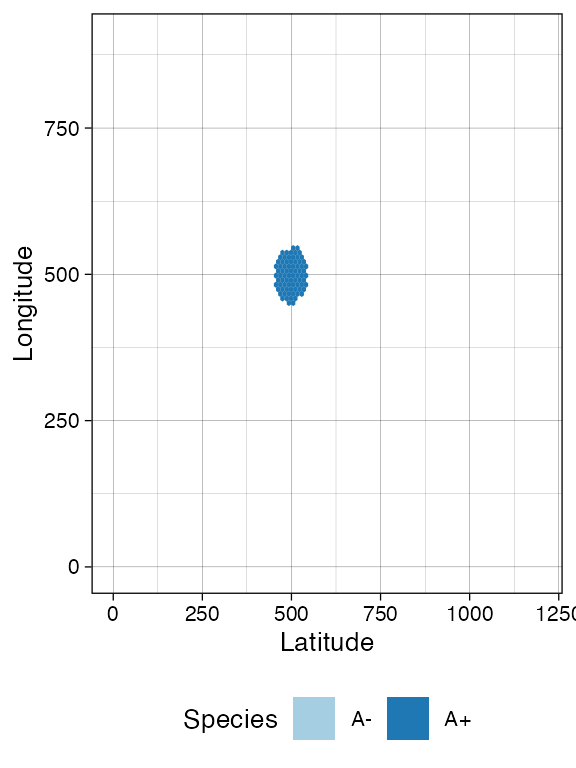
Getting Cells (Advanced)
At this point, if we query the simulation we will find more cells (we
use dplyr to process query results). For convenience, the
getters accept parameters to subset the tissue.
# load dplyr to use %>%
require(dplyr)

# Get the cells in the tissue at current simulation time
sim$get_cells() %>% head()
#>   cell_id mutant epistate position_x position_y
#> 1   21730      A        +        458        497
#> 2   21697      A        +        458        498
#> 3   19846      A        +        459        483
#> 4   18816      A        +        459        489
#> 5   20217      A        -        459        494
#> 6   21729      A        +        459        497

# Get the cells in the tissue rectangular sample having
# [500,500] and [505,505] as lower and upper corners, respectively
sim$get_cells(c(500, 500), c(505, 505))  %>% head()
#>   cell_id mutant epistate position_x position_y
#> 1   12150      A        +        500        500
#> 2   20546      A        +        500        501
#> 3   17481      A        +        500        502
#> 4   17482      A        +        500        503
#> 5   20091      A        -        500        504
#> 6   19642      A        +        500        505

# Get the cells in the tissue having epigenetic state "-"
sim$get_cells(c("A", "B"), c("-")) %>% head()
#>   cell_id mutant epistate position_x position_y
#> 1   20217      A        -        459        494
#> 2   21494      A        -        459        504
#> 3   20144      A        -        460        484
#> 4   20218      A        -        460        493
#> 5   18519      A        -        460        496
#> 6   21493      A        -        460        504

# Get the cells in the tissue having epigenetic state "-" and,
# at the same time, belonging to rectangular sample bounded by
# [500,500] and [505,505] as lower and upper corners, respectively
sim$get_cells(c(500, 500), c(505, 505), c("A", "B"), c("-"))  %>% head()
#>   cell_id mutant epistate position_x position_y
#> 1   20091      A        -        500        504
#> 2    9405      A        -        502        500
#> 3   21653      A        -        502        504
#> 4   21654      A        -        503        505
#> 5    4689      A        -        505        502
Evolving new species
rRACES can select cells from the tissue, randomly for every mutant, or in a constrained tissue area.
# Stochastic sampling from the whole tissue: it can return A+ or A-
sim$choose_cell_in("A")
#>   cell_id mutant epistate position_x position_y
#> 1   21730      A        +        458        497

# Calling it again may result in a different cell
sim$choose_cell_in("A")
#>   cell_id mutant epistate position_x position_y
#> 1   21546      A        +        492        455

# Constrain sampling in the tissue rectangular selection [500,550]x[350,450]
sim$choose_cell_in("A",  c(500, 350), c(550, 450))
#>   cell_id mutant epistate position_x position_y
#> 1   17516      A        +        494        456
This feature can be used to program the generation of new species, mimicking new mutants that generate subclonal expansions.
Imagine we want to add a new mutant B with epistates –
and therefore new species B+ and B- - as
descending from A,we need to:
locate one cell of mutant
Ain the tissue, which is where we will inject the new mutant;add the specifics of mutant
B(viaSpatialSimulation$add_mutant(), as we did forA);implement the change of the cell of mutant
Ato a cell of mutantB.
# We locate a random cell
cell <- sim$choose_cell_in("A")
cell
#>   cell_id mutant epistate position_x position_y
#> 1   21546      A        +        492        455

# Add mutant
sim$add_mutant(name = "B",
               epigenetic_rates = c("+-" = 0.05, "-+" = 0.05),
               growth_rates = c("+" = 0.7, "-" = 0.3),
               death_rates = c("+" = 0.05, "-" = 0.1))
Then we inject the cell, and simulate a little bit.
# Mutant injection
sim$mutate_progeny(cell, "B")

# Generated event A -> B either in + or - epistates is now recorded
sim$get_counts()
#>   mutant epistate counts overall
#> 1      A        -   1008    3146
#> 2      A        +   4162   24669
#> 3      B        -      0       0
#> 4      B        +      1       1

# New evolution
sim$run_up_to_size("B+", 600)
#>  [████████████████████████████████████████] 100% [00m:00s] Saving snapshot
At this point, we can inspect in more details the tissue. It can help to facet on the species to clearly appreciate the spatial diffusion of the populations.
plot_state(sim)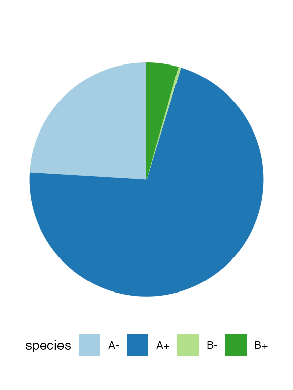
plot_tissue(sim, num_of_bins = 250)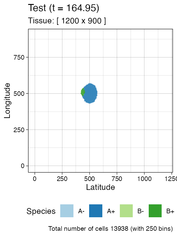
# Facet on species via ggplot
library(ggplot2)

plot_tissue(sim, num_of_bins = 250) + facet_wrap(~species)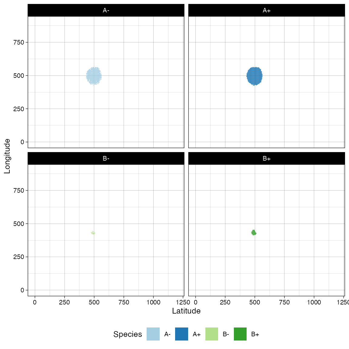
If, at this point in the simulation, we generate a new mutant
C from A in the rectangle
.
# Define evolutionary parameters
sim$add_mutant(name = "C",
               epigenetic_rates = c("+-" = 0.1, "-+" = 0.1),
               growth_rates = c("+" = 0.2, "-" = 0.4),
               death_rates = c("+" = 0.1, "-" = 0.01))

# Choose and mutate
sim$mutate_progeny(sim$choose_cell_in("A",  c(450, 550), c(500, 600)), "C")

sim$run_up_to_time(sim$get_clock() + 7)
#>  [████████████████████████████████████████] 100% [00m:00s] Saving snapshot
plot_state(sim)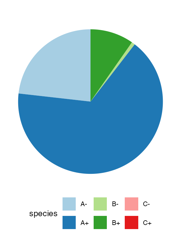
plot_tissue(sim, num_of_bins = 250)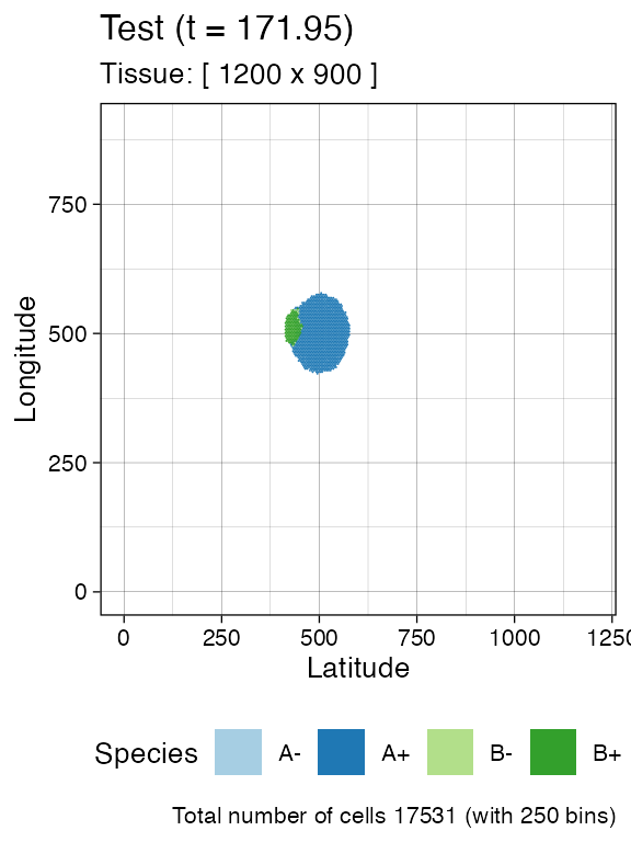
Other Operations
Injection of Cells over a Tissue
On the tissue, we can inject multiple cells manually; all injected cells can be retrieved.
# Now it will return just the initial cell
sim$get_added_cells()
#>   mutant epistate position_x position_y time
#> 1      A        +        500        500    0
Avoiding Drift
Any species that has a non-zero death rate can become extinct stochastically by drift.
Drift makes it difficult to simulate an be confident of what species are in the model. To facilitate the user, RACES can avoid drift by setting a death activation level. This value is the minimum number of cells that enables cell death in a species: a cell of species can die if and only if has reached the death activation level at least once during the simulation.
This threshold holds for all the species and it is set to 1 by default.
sim$death_activation_level
#> [1] 1

# Change death activation level
sim$death_activation_level <- 50