2. Survival analysis of the MSK-MetTropism Cohort
Source:vignettes/a2_survival_analysis.Rmd
a2_survival_analysis.Rmd
library(INCOMMON)
#> Warning: replacing previous import 'cli::num_ansi_colors' by
#> 'crayon::num_ansi_colors' when loading 'INCOMMON'
library(dplyr)
#>
#> Attaching package: 'dplyr'
#> The following objects are masked from 'package:stats':
#>
#>     filter, lag
#> The following objects are masked from 'package:base':
#>
#>     intersect, setdiff, setequal, union
In this vignette we carry out survival analysis based on INCOMMON classification of samples of pancreatic adenocarcinoma (PAAD) patients of the MSK-MetTropsim cohort.
First we prepare the input using function init:
data(MSK_genomic_data)
data(MSK_clinical_data)
data(cancer_gene_census)

x = init(
  genomic_data = MSK_genomic_data,
  clinical_data = MSK_clinical_data %>% filter(tumor_type == 'PAAD'),
  gene_roles = cancer_gene_census
)
#> ── INCOMMON - Inference of copy number and mutation multiplicity in oncology ───
#>
#> ── Genomic data ──
#>
#> ✔ Found 25659 samples, with 224939 mutations in 491 genes
#> ! No read counts found for 1393 mutations in 1393 samples
#> ! Gene name not provided for 1393 mutations
#> ! 201 genes could not be assigned a role (TSG or oncogene)
#>
#> ── Clinical data ──
#>
#> ℹ Provided clinical features:
#> ✔ sample (required for classification)
#> ✔ purity (required for classification)
#> ✔ tumor_type
#> ✔ OS_MONTHS
#> ✔ OS_STATUS
#> ✔ SAMPLE_TYPE
#> ✔ MET_COUNT
#> ✔ METASTATIC_SITE
#> ✔ MET_SITE_COUNT
#> ✔ PRIMARY_SITE
#> ✔ SUBTYPE_ABBREVIATION
#> ✔ GENE_PANEL
#> ✔ TMB_NONSYNONYMOUS
#> ✔ FGA
#> ✔ AGE_AT_DEATH
#> ✔ Found 1742 matching samples
#> ✖ Found 23917 unmatched samples

print(x)
#> ── [ INCOMMON ]  6779 PASS mutations across 1740 samples, with 276 mutant genes
#> ℹ Average sample purity: 0.26
#> ℹ Average sequencing depth: 623
#> # A tibble: 6,779 × 25
#>    sample   tumor_type purity chr     from     to ref   alt      DP    NV    VAF
#>    <chr>    <chr>       <dbl> <chr>  <dbl>  <dbl> <chr> <chr> <int> <int>  <dbl>
#>  1 P-00094… PAAD          0.1 chr12 2.54e7 2.54e7 C     T       847    82 0.0968
#>  2 P-00094… PAAD          0.1 chr17 7.58e6 7.58e6 C     T       709    91 0.128
#>  3 P-00215… PAAD          0.4 chr12 2.54e7 2.54e7 C     T      1048   322 0.307
#>  4 P-00215… PAAD          0.4 chr17 7.57e6 7.57e6 G     A       942   384 0.408
#>  5 P-00215… PAAD          0.4 chr1  2.71e7 2.71e7 -     G       833   289 0.347
#>  6 P-00215… PAAD          0.4 chr1  1.13e7 1.13e7 T     C      1115   300 0.269
#>  7 P-00215… PAAD          0.4 chr3  1.87e8 1.87e8 G     A      1362   847 0.622
#>  8 P-00034… PAAD          0.2 chr12 2.54e7 2.54e7 C     T       533    56 0.105
#>  9 P-00034… PAAD          0.2 chr17 7.58e6 7.58e6 C     A       351    56 0.160
#> 10 P-00245… PAAD          0.2 chr12 2.54e7 2.54e7 C     G       938   155 0.165
#> # ℹ 6,769 more rows
#> # ℹ 14 more variables: gene <chr>, gene_role <chr>, OS_MONTHS <dbl>,
#> #   OS_STATUS <dbl>, SAMPLE_TYPE <chr>, MET_COUNT <dbl>, METASTATIC_SITE <chr>,
#> #   MET_SITE_COUNT <dbl>, PRIMARY_SITE <chr>, SUBTYPE_ABBREVIATION <chr>,
#> #   GENE_PANEL <chr>, TMB_NONSYNONYMOUS <dbl>, FGA <dbl>, AGE_AT_DEATH <dbl>
There are 6779 mutations with average sequencing depth 623 across 1740 samples with average purity 0.26.
Classification of 1740 pancreatic adenocarcinoma samples
We then classify the mutations using PCAWG priors and the default entropy cutoff and overdispersion parameter:
x = classify(
  x = x,
  priors = pcawg_priors,
  entropy_cutoff = 0.2,
  rho = 0.01
)
print(x)
#> ── [ INCOMMON ]  6779 PASS mutations across 1740 samples, with 276 mutant genes
#> ℹ Average sample purity: 0.26
#> ℹ Average sequencing depth: 623
#> ── [ INCOMMON ]  Classified mutations with overdispersion parameter 0.01 and ent
#> # A tibble: 6,779 × 18
#>    sample   tumor_type purity chr     from     to ref   alt      DP    NV    VAF
#>    <chr>    <chr>       <dbl> <chr>  <dbl>  <dbl> <chr> <chr> <int> <int>  <dbl>
#>  1 P-00094… PAAD          0.1 chr12 2.54e7 2.54e7 C     T       847    82 0.0968
#>  2 P-00094… PAAD          0.1 chr17 7.58e6 7.58e6 C     T       709    91 0.128
#>  3 P-00215… PAAD          0.4 chr12 2.54e7 2.54e7 C     T      1048   322 0.307
#>  4 P-00215… PAAD          0.4 chr17 7.57e6 7.57e6 G     A       942   384 0.408
#>  5 P-00215… PAAD          0.4 chr1  2.71e7 2.71e7 -     G       833   289 0.347
#>  6 P-00215… PAAD          0.4 chr1  1.13e7 1.13e7 T     C      1115   300 0.269
#>  7 P-00215… PAAD          0.4 chr3  1.87e8 1.87e8 G     A      1362   847 0.622
#>  8 P-00034… PAAD          0.2 chr12 2.54e7 2.54e7 C     T       533    56 0.105
#>  9 P-00034… PAAD          0.2 chr17 7.58e6 7.58e6 C     A       351    56 0.160
#> 10 P-00245… PAAD          0.2 chr12 2.54e7 2.54e7 C     G       938   155 0.165
#> # ℹ 6,769 more rows
#> # ℹ 7 more variables: gene <chr>, gene_role <chr>, id <chr>, label <chr>,
#> #   state <chr>, posterior <dbl>, entropy <dbl>
There are 2611 heterozygous diploid mutations (HMD), 558 mutations with loss of heterozygosity (LOH), 1988 mutations with copy-neutral LOH (CNLOH), 283 mutations with amplification. In addition, 1339 mutations were classified as Tier-2, either because of entropy being larger than cutoff or because of a low number of mutant alleles relative to the wild-type.
Genome interpretation
INCOMMON provides a function to aid the interpretation of the mutant genome, downstream of classification. Full inactivation of tumor suppressor genes (TSG) are detected as mutations wiht loss of the wild-type allele, either through pure loss of heterozygosity (LOH) or with copy-neutral LOH (CNLOJ). Enhanced activation of oncogenes are identified as mutations with amplification of the mutant allele. In addition to amplifications in trisomy and tetrasomy (AM), CNLOH events are interpreted for oncogenes as amplifications in disomy, since the mutant allele is found in double copy.
The function genome_interpreter adds two variables to
the classification object: the class,
indicating for each mutant gene whether it is with LOH or amplification,
depending on the gene role. In addition, each sample is annotated with a
genotype that summarises all the interpreted mutation found
in the sample.
x = genome_interpreter(x = x)
#> ℹ There are 1288 different genotypes
#> ℹ The most abundant genotypes are:
#> • Mutant KRAS without AMP,Mutant TP53 without LOH (59 Samples, Frequency 0.03)
#> • Mutant KRAS with AMP,Mutant TP53 with LOH (53 Samples, Frequency 0.03)
#> • Mutant KRAS without AMP (44 Samples, Frequency 0.03)
Across the PAAD samples that we classified, there are 1288 different genotypes, the most abundant ones being different combinations of TP53 with/without LOH and KRAS mutations with/without amplifications.
Survival analysis of Mutant KRAS patients
We can investigate the impact on patients’ survival of a target class, for example Mutant KRAS with/without amplification, with respect to KRAS WT patients.
We first look at the distribution of INCOMMON copy number states
across PAAD samples for KRAS, using function
plot_class_fraction:
plot_class_fraction(x = x, tumor_type = 'PAAD', gene = 'KRAS')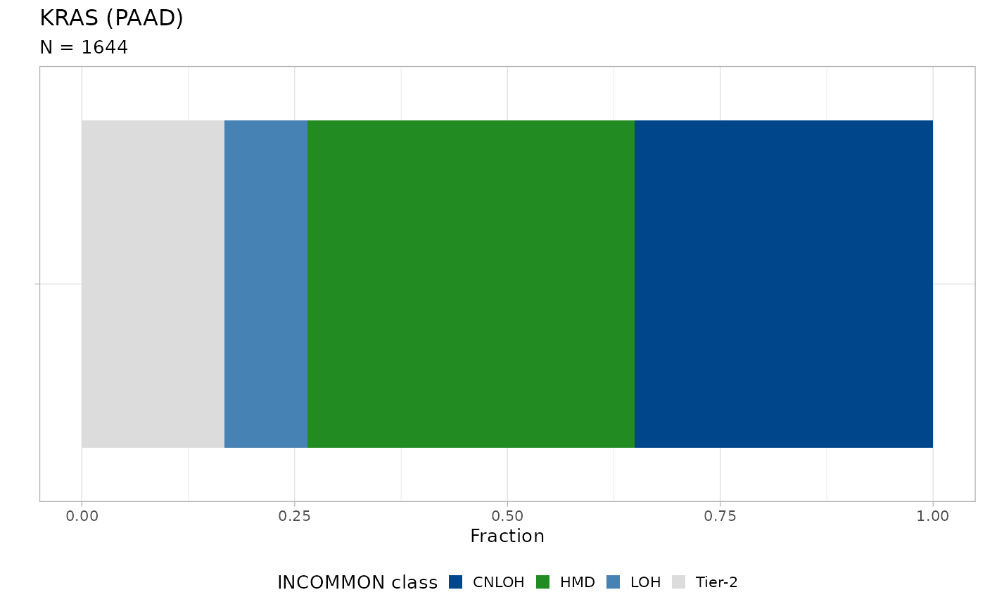 Nearly 30% of KRAS mutations are associated with amplification of the
mutant allele, mostly through CNLOH (multiplicity \(m=2\) in disomy).
Nearly 30% of KRAS mutations are associated with amplification of the
mutant allele, mostly through CNLOH (multiplicity \(m=2\) in disomy).
We can compare the INCOMMON posterior distribution with the utilised prior from PCAWG:
plot_prior(x = pcawg_priors, gene = 'KRAS', tumor_type = 'PAAD')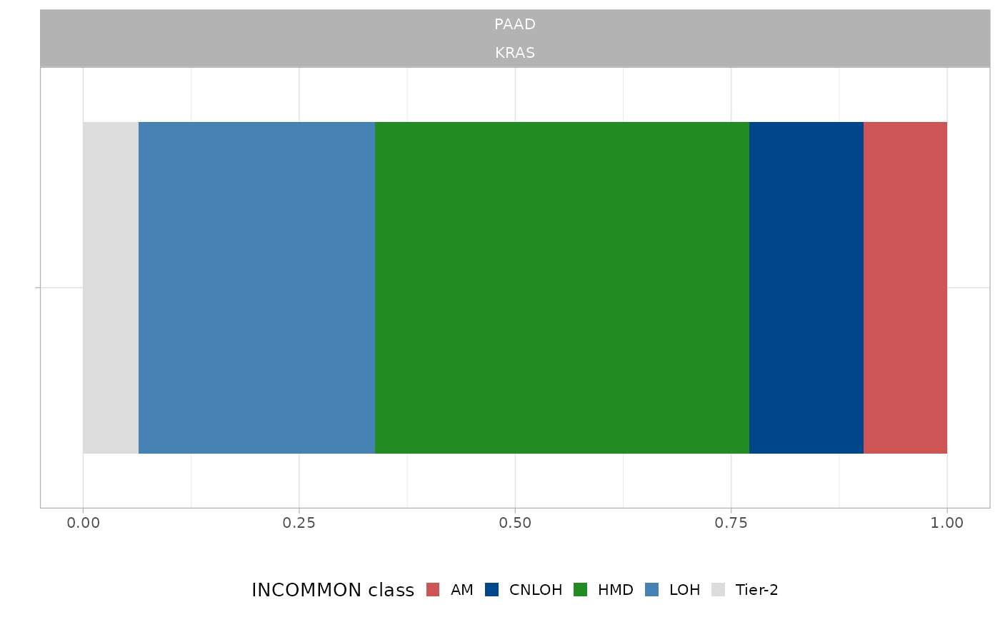
A PAAD-specific prior is available. By comparing the two plots, we can see that , with respect to PCAWG, in Mutant KRAS PAAD samples from the MSK-MetTropism cohort there is an evident increase of amplifications in disomy (CNLOH), whereas no trisomy or tetrasomy amplifications (AM) are detected. There is also an under-representation of pure LOH states, whereas the fraction of heterozygous diploid mutations is quite similar.
Next we use function kaplan_meier_fit to fit survival
data (overall survival status versus overall survival months) using the
Kaplan-Meier estimator.
x = kaplan_meier_fit(x = x, tumor_type = 'PAAD', gene = 'KRAS')
#> Call: survfit(formula = survival::Surv(OS_MONTHS, OS_STATUS) ~ group,
#>     data = data)
#>
#>                           n events median 0.95LCL 0.95UCL
#> KRAS WT                 109     63   21.5   18.86    30.8
#> Mutant KRAS without AMP 626    391   18.1   15.84    20.7
#> Mutant KRAS with AMP    573    394   11.7    9.69    13.2
The median survival time decreases from 21.5 months for the KRAS WT group to 18.2 months for Mutant KRAS without amplification and further to 11.7 months for Mutant KRAS with amplification patients.
In order to estimate the hazard ratio associated with these groups, we fit the same survival data, this time using a multivariate Cox proportional hazards regression model. Here, we include the age of patients at death, sex and tumor mutational burden as model covariates.
x = cox_fit(x = x,
        tumor_type = 'PAAD',
        gene = 'KRAS',
        survival_time = 'OS_MONTHS',
        survival_status = 'OS_STATUS',
        covariates = c('age', 'sex', 'tmb'))
#> Call:
#> survival::coxph(formula = formula %>% as.formula(), data = data %>%
#>     as.data.frame())
#>
#>                                  coef exp(coef) se(coef)      z      p
#> groupMutant KRAS with AMP     0.34419   1.41085  0.13798  2.495 0.0126
#> groupMutant KRAS without AMP  0.03665   1.03733  0.13762  0.266 0.7900
#> AGE_AT_DEATH>67              -0.12559   0.88197  0.07054 -1.781 0.0750
#> TMB_NONSYNONYMOUS>4           0.14600   1.15719  0.07035  2.075 0.0380
#>
#> Likelihood ratio test=28.06  on 4 df, p=1.214e-05
#> n= 838, number of events= 838
#>    (470 observations deleted due to missingness)
This analysis reveals that, whereas KRAS mutation alone (without amplification) is not enough, the presence of amplification significantly increases the hazard ratio (HR = 1.41, p-value = 0.012) with respect to the WT group. Moreover, tumor mutational burden (TMB_NONSYNONYMOUS) also gives a significant albeit weak contribution, as patients with more than 4 non-synonymous mutations (median TMB_NONSYNONYMOUS) emerge as being more at risk (HR = 1.16, p-value = 0.038).
Kaplan-Meier estimation and multivariate Cox regression can be
visualized straightforwardly using the
plot_survival_analysis function:
plot_survival_analysis(x = x,
                       tumor_type = 'PAAD',
                       gene = 'KRAS')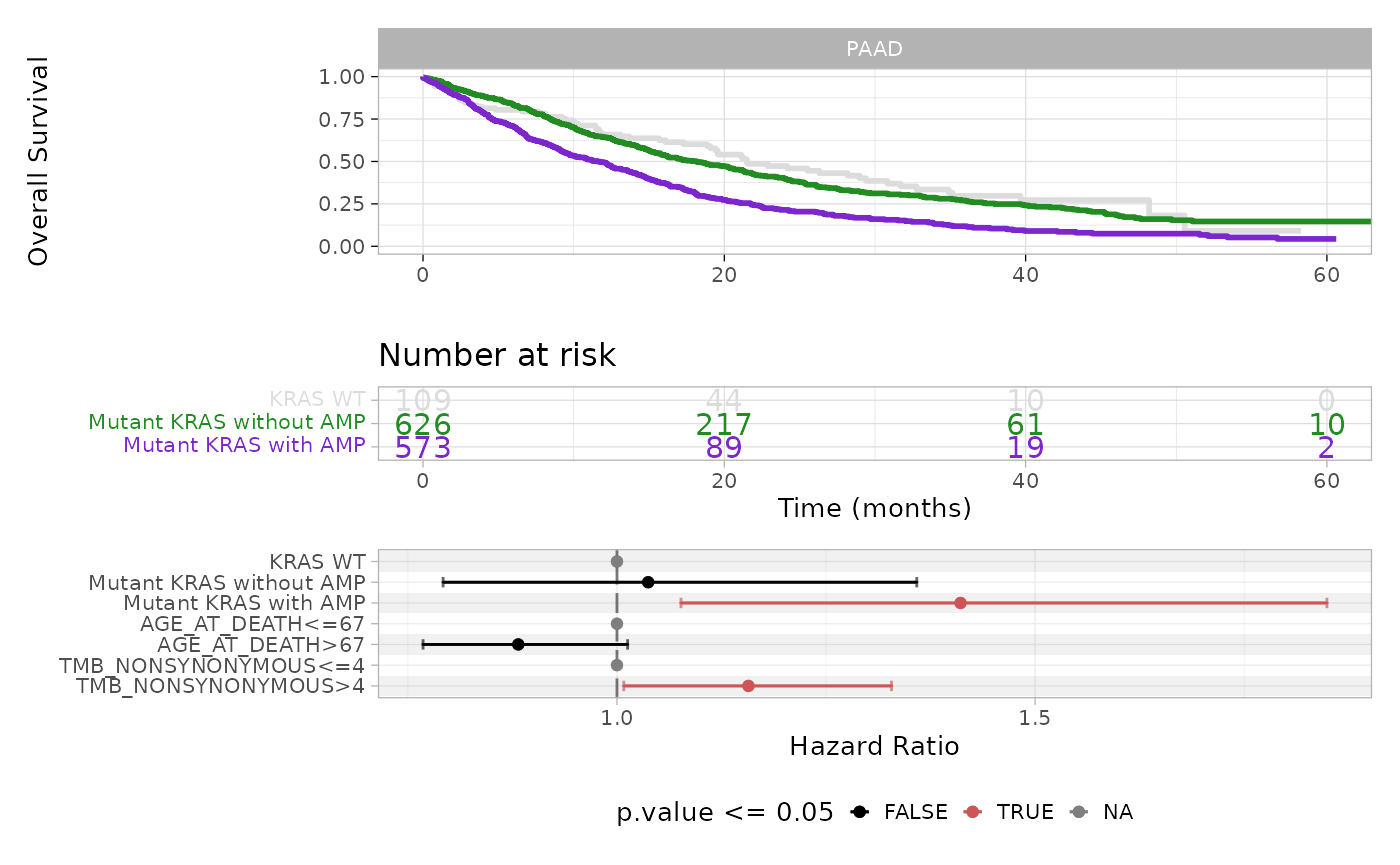
The plot displays Kaplan-Meier survival curves and risk table, and a forest plot for Cox multivariate regression coefficients, highlighting in red the covariates that have a statistically significant contribution to differences in hazard risks.