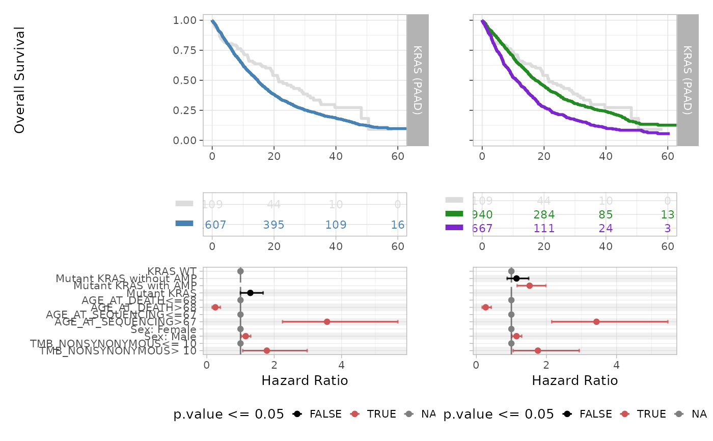
Visualise survival analysis based on INCOMMON classes.

Usage

plot_survival_analysis(
  x,
  tumor_type,
  gene,
  cox_covariates = c("age", "sex", "tmb")
)

Arguments

x: A list of objects of class 'INCOMMON' containing the classification results for multiple samples, as produced by using function classify.
tumor_type: The selected tumour type.
gene: The selected gene.
cox_covariates: A character vector listing the covariates to be used in the multivariarte regression.

Value

An object or a list of class 'ggplot2' showing Kaplan-Meier curves and Cox regression forest plot.

Examples

# First load example classified data
data(MSK_PAAD_output)
# Perform survival analysis based on the classification of KRAS mutant samples of pancreatic adenocarcinoma
MSK_PAAD_output = kaplan_meier_fit(x = MSK_PAAD_output, tumor_type = 'PAAD', gene = 'KRAS', survival_time = 'OS_MONTHS', survival_status = 'OS_STATUS')
#> Joining with `by = join_by(id)`
#> Call: survfit(formula = "survival::Surv(OS_MONTHS, OS_STATUS) ~ group", 
#>     data = data)
#> 
#>    7 observations deleted due to missingness 
#>                   n events median 0.95LCL 0.95UCL
#> WT              214     92   38.3   28.98    51.1
#> Low Dosage      541    344   17.4   15.34    19.8
#> Balanced Dosage 670    417   14.6   13.34    15.8
#> High Dosage     347    237   10.7    9.36    12.5
# Perform Cox regression
MSK_PAAD_output = cox_fit(x = MSK_PAAD_output, tumor_type = 'PAAD', gene = 'KRAS', survival_time = 'OS_MONTHS', survival_status = 'OS_STATUS', covariates = c('age', 'sex', 'tmb'), tmb_method = ">10")
#> [1] "Cox fit with INCOMMON groups:"
#> Call:
#> survival::coxph(formula = formula %>% stats::as.formula(), data = data %>% 
#>     as.data.frame())
#> 
#>                        coef exp(coef) se(coef)     z        p
#> groupBalanced Dosage 0.8179    2.2658   0.1159 7.058 1.69e-12
#> groupHigh Dosage     1.1569    3.1801   0.1242 9.318  < 2e-16
#> groupLow Dosage      0.6840    1.9818   0.1177 5.810 6.24e-09
#> 
#> Likelihood ratio test=102.1  on 3 df, p=< 2.2e-16
#> n= 1772, number of events= 1090 
#>    (7 observations deleted due to missingness)
#> [1] "Pairwise tests:"
#> 
#> 	 Simultaneous Tests for General Linear Hypotheses
#> 
#> Fit: survival::coxph(formula = formula %>% stats::as.formula(), data = data %>% 
#>     as.data.frame())
#> 
#> Linear Hypotheses:
#>                                                  Estimate Std. Error z value
#> `groupHigh Dosage` - `groupBalanced Dosage` == 0  0.33900    0.08156   4.156
#> `groupLow Dosage` - `groupBalanced Dosage` == 0  -0.13391    0.07299  -1.835
#>                                                  Pr(>|z|)    
#> `groupHigh Dosage` - `groupBalanced Dosage` == 0 6.45e-05 ***
#> `groupLow Dosage` - `groupBalanced Dosage` == 0     0.123    
#> ---
#> Signif. codes:  0 ‘***’ 0.001 ‘**’ 0.01 ‘*’ 0.05 ‘.’ 0.1 ‘ ’ 1
#> (Adjusted p values reported -- single-step method)
#> 
plot_survival_analysis(x = MSK_PAAD_output, tumor_type = 'PAAD', gene = 'KRAS')
#> Scale for x is already present.
#> Adding another scale for x, which will replace the existing scale.
#> Scale for x is already present.
#> Adding another scale for x, which will replace the existing scale.
#> Joining with `by = join_by(var)`
#> Joining with `by = join_by(var)`
#> Warning: Removed 3 rows containing missing values or values outside the scale range
#> (`geom_rect()`).
#> Warning: Removed 3 rows containing missing values or values outside the scale range
#> (`geom_point()`).
#> Warning: Removed 1 row containing missing values or values outside the scale range
#> (`geom_rect()`).
#> Warning: Removed 1 row containing missing values or values outside the scale range
#> (`geom_point()`).