Object Initialization and preprocessing
Source:vignettes/1_create_congas_object.Rmd
1_create_congas_object.RmdIn this Vignette we show how to create a CONGAS+ object starting from RNA and ATAC count matrices. We will use the B-cell lymphoma cells sequences via 10x genomics multiomic assay. The raw data can be foun here. Setup the directory where results are stored.
sample = 'lymphoma'

prefix = paste0(sample, "/tutorial/")

out.dir = paste0(prefix, "/congas_data/")
fig.dir = paste0(prefix, "/congas_figures/")

if (!dir.exists(out.dir)) {dir.create(out.dir, recursive = T)}
if (!dir.exists(fig.dir)) {dir.create(fig.dir, recursive = T)}
Load the ATAC counts to create the tibble needed as CONGAS+ input
With the multiome assay, the feature files provided by CellRanger contains already a mapping between gene names and coordinates. Let’s read this file As an alternative, when such file not not readily available, users can exploit BiomaRt. Please see the correspodning vignette
data(features)Create the RNA and ATAC tibble required by CONGAS+
atac_featureDF = data.frame(id = rownames(atac_counts)) %>%
  tidyr::separate(id, c('chr', 'from', 'to'), '-')

atac = Rcongas::create_congas_tibble(counts = atac_counts,
                                     modality = 'ATAC',
                                     save_dir = NULL,
                                     features = atac_featureDF)
#> ℹ Saving temporary counts file
#> Rows: 3100055 Columns: 3
#> ── Column specification ────────────────────────────────────────────────────────
#> Delimiter: " "
#> dbl (3): 109788, 500, 3100055
#>
#> ℹ Use `spec()` to retrieve the full column specification for this data.
#> ℹ Specify the column types or set `show_col_types = FALSE` to quiet this message.
#> Joining with `by = join_by(feature_index)`
#> Joining with `by = join_by(cell_index)`

# Compute normalization factors
norm_atac = Rcongas:::auto_normalisation_factor(atac) %>%
  mutate(modality = 'ATAC')
#> → Computing library size factors as total counts.
#> → Median digits per factor 4.5, scaling by 31622.7766016838.
#>    Min. 1st Qu.  Median    Mean 3rd Qu.    Max.
#>  0.0309  0.1610  0.3184  0.4383  0.5927  2.1472

rna = Rcongas::create_congas_tibble(counts = rna_counts,
                                    modality = 'RNA',
                                    save_dir=NULL,
                                    features = features)
#> ℹ Saving temporary counts file
#> Rows: 1049590 Columns: 3── Column specification ────────────────────────────────────────────────────────
#> Delimiter: " "
#> dbl (3): 36601, 500, 1049590
#> ℹ Use `spec()` to retrieve the full column specification for this data.
#> ℹ Specify the column types or set `show_col_types = FALSE` to quiet this message.Joining with `by = join_by(feature_index)`Joining with `by = join_by(cell_index)`


# Compute normalization factors
norm_rna = Rcongas:::auto_normalisation_factor(rna) %>%
  mutate(modality = 'RNA')
#> → Computing library size factors as total counts.
#> → Median digits per factor 4, scaling by 10000.
#>    Min. 1st Qu.  Median    Mean 3rd Qu.    Max.
#>  0.0627  0.1671  0.2724  0.3964  0.4966  2.4000

atac = atac %>% mutate(value = as.integer(value))
rna = rna %>% mutate(value = as.integer(value))
Apply some basic filters on known genes
rna = rna %>% filter_known_genes(what='r')
#>
#> ── Ribosomal
#> ℹ n = 185 genes found.
#> RPL22, RPL11, RPS6KA1, RPS8, MRPL37, RPL5 , ...
#>
#> ── Specials
#> ℹ n = 1 genes found.

all_genes = rna$gene %>% unique
mito = all_genes %>% str_starts(pattern = 'MT-')
all_genes = setdiff(all_genes, all_genes[mito])
rna = rna %>% dplyr::filter(gene %in% all_genes)
Read chromosome arm coordinated that will be used as segment breakpoints
data(example_segments)

# Remove these chromosomes
segments = example_segments %>% dplyr::filter(chr != 'chrX', chr != 'chrY')
Now init the (R)CONGAS+ object. Users can choose between two object types: the multiomic or standard CONGAS+, setting the parameter to TRUE or FALSE, respectively. When the observations between RNA and ATAC are paired, the multiomic object should be used, in order to assign the RNA and ATAC observations from the same cells to the same clusters. Please note that in this case the cells are expected to have the same barcode in the two modalities. The object provided as an example in this vignette illustrates this.
x = init(
  rna = rna,
  atac = atac,
  segmentation = segments, #%>% mutate(copies = as.integer(round(copies))),
  rna_normalisation_factors = norm_rna,
  atac_normalisation_factors = norm_atac,
  rna_likelihood = "NB",
  atac_likelihood = "NB",
  description = paste0('Bimodal ', sample),
  multiome = TRUE)
#>                        ┌──────────────────────────────────┐
#>                        │                                  │
#>                        │   (R)CONGAS+: Bimodal lymphoma   │
#>                        │                                  │
#>                        └──────────────────────────────────┘
#> [1] "Running in multiome mode."
#>
#> ── RNA modality (46.631816 Mb)
#> → Input events: 1028900
#> → Input cells: 500
#> → Input locations: 21771
#> → Cleaning outlier features from RNA input matrix
#> → Normalising RNA counts using input normalisation factors.
#> Warning: The `<scale>` argument of `guides()` cannot be `FALSE`. Use "none" instead as
#> of ggplot2 3.3.4.
#> ℹ The deprecated feature was likely used in the Rcongas package.
#>   Please report the issue to the authors.
#> This warning is displayed once every 8 hours.
#> Call `lifecycle::last_lifecycle_warnings()` to see where this warning was
#> generated.
#> → Found: 109 outliers.
#> → Entries mapped: 491441, with 537459 outside input segments that will be discarded.
#> → Using likelihood: NB.
#> Joining with `by = join_by(cell)`
#>
#> ── ATAC modality (111.685272 Mb)
#> → Input events: 3100055
#> → Input cells: 500
#> → Input locations: 109645
#> → Cleaning outlier features from ATAC input matrix
#> Joining with `by = join_by(chr, from, to)`→ Normalising ATAC counts using input normalisation factors.
#> → Found: 581 outliers.
#> → Entries mapped: 1530455, with 1569600 outside input segments that will be discarded.
#> → Using likelihood: NB.
#> Joining with `by = join_by(cell)`
#> ── Checking segmentation
#> ! These segments have no events associated and will be removed - we suggest you to check if these can be further smoothed.
#> ℹ  Hint  Check if the reduced segments can be further smoothed!
#> # A tibble: 3 × 11
#>   chr    from       to copies segment_id      RNA_nonzerocells ATAC_nonzerocells
#>   <chr> <int>    <int>  <int> <chr>                      <dbl>             <dbl>
#> 1 chr13     0 17700000      2 chr13:0:177000…                0                 0
#> 2 chr14     0 17200000      2 chr14:0:172000…                0                 0
#> 3 chr15     0 19000000      2 chr15:0:190000…                0                 0
#> # ℹ 4 more variables: ATAC_nonzerovals <dbl>, ATAC_peaks <dbl>,
#> #   RNA_nonzerovals <dbl>, RNA_genes <dbl>
#> ✖ Warning RNA 0-counts cells. 374 cells have missing data in any of 23 segments, top 5 with missing data are:
#> ✖ Cell AAACCGAAGTGGACAA-1-RNA with 1 0-segments (4%)
#> ✖ Cell AAACGCGCAGGTTCAC-1-RNA with 1 0-segments (4%)
#> ✖ Cell AAACGTACATAATGAG-1-RNA with 1 0-segments (4%)
#> ✖ Cell AAAGGTTAGGCCAATT-1-RNA with 1 0-segments (4%)
#> ✖ Cell AACATTGTCCTACCTA-1-RNA with 1 0-segments (4%)
#> ✖ Warning ATAC 0-counts cells. 209 cells have no data in any of 23 segments, top 5 with missing data are:
#> ✖ Cell GTCCTAGAGCCAAATC-1-ATAC with 2 0-segments (9%)
#> ✖ Cell TCTCGCCCAAACATAG-1-ATAC with 2 0-segments (9%)
#> ✖ Cell AAACGCGCAGGTTCAC-1-ATAC with 1 0-segments (4%)
#> ✖ Cell AAACGTACATAATGAG-1-ATAC with 1 0-segments (4%)
#> ✖ Cell AAAGCCGCATAGTCAT-1-ATAC with 1 0-segments (4%)
Now plot the number of nonzero cells vs the number of peaks per segment, to help identify a threshold for filtering segments.
ggplot(x$input$segmentation, aes(x=ATAC_nonzerocells, y=ATAC_peaks)) + geom_point() + theme_bw()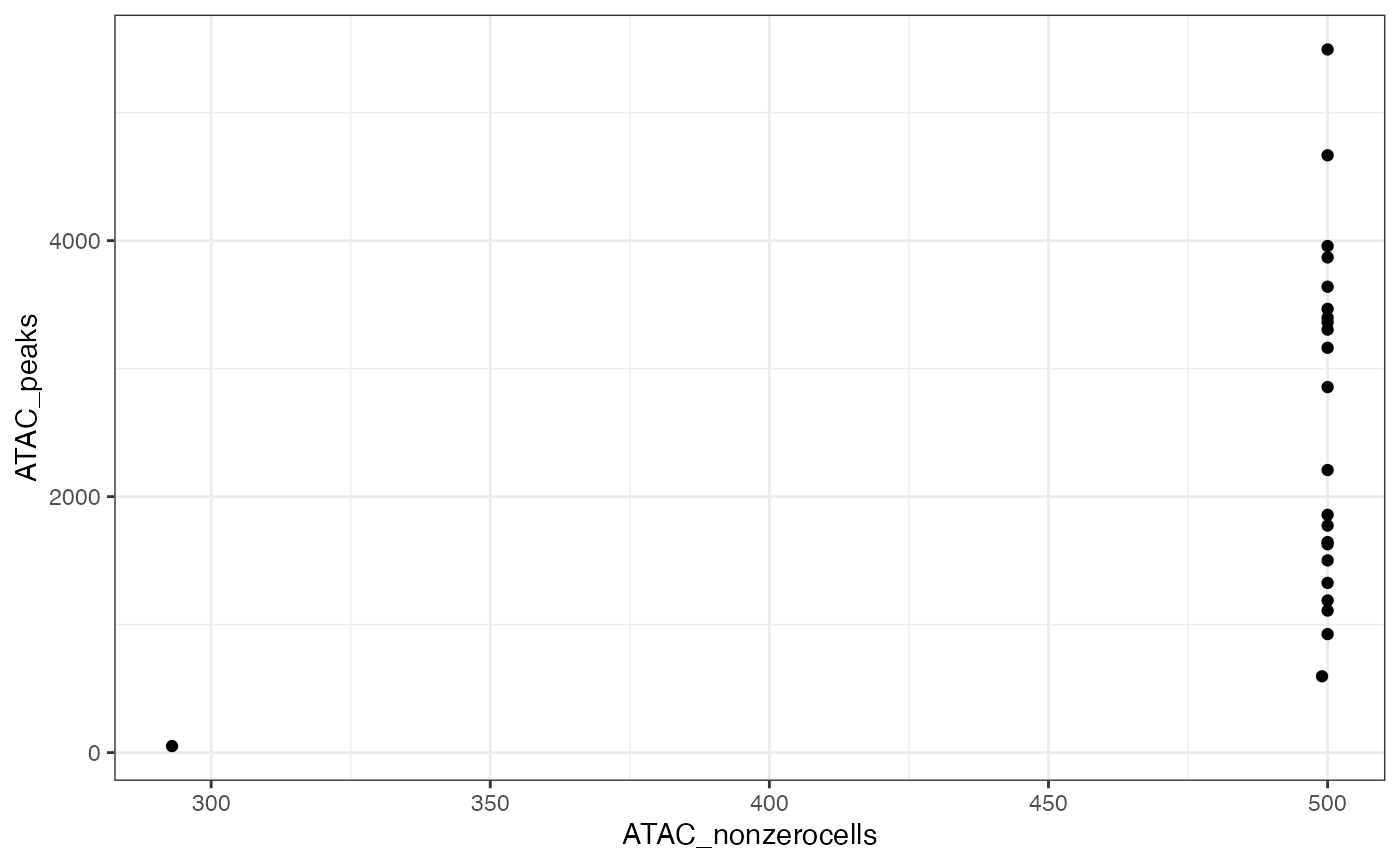
ggplot(x$input$segmentation, aes(x=RNA_nonzerocells, y=RNA_genes)) + geom_point() + theme_bw()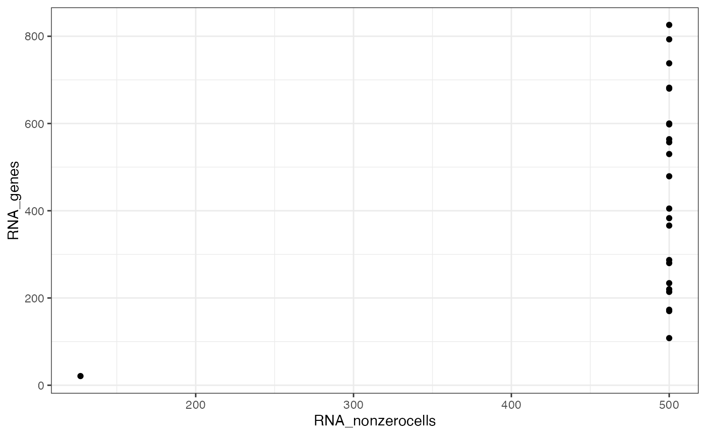
x = Rcongas::filter_segments(x, RNA_nonzerocells = 300, ATAC_nonzerocells = 300)
#>
#> ── Segments filter
#> → 22 retained segments out of 23.
Generate plots to check out the data distribution
plot_data(
  x,
  what = 'histogram',
  segments = get_input(x, what = 'segmentation') %>%
    ungroup() %>%
    mutate(L = to - from) %>%
    dplyr::arrange(dplyr::desc(L)) %>%
    dplyr::top_n(9) %>%
    pull(segment_id)
)
#> → Normalising RNA counts using input normalisation factors.
#> → Normalising ATAC counts using input normalisation factors.
#> Selecting by L
#> → Showing all segments (this plot can be large).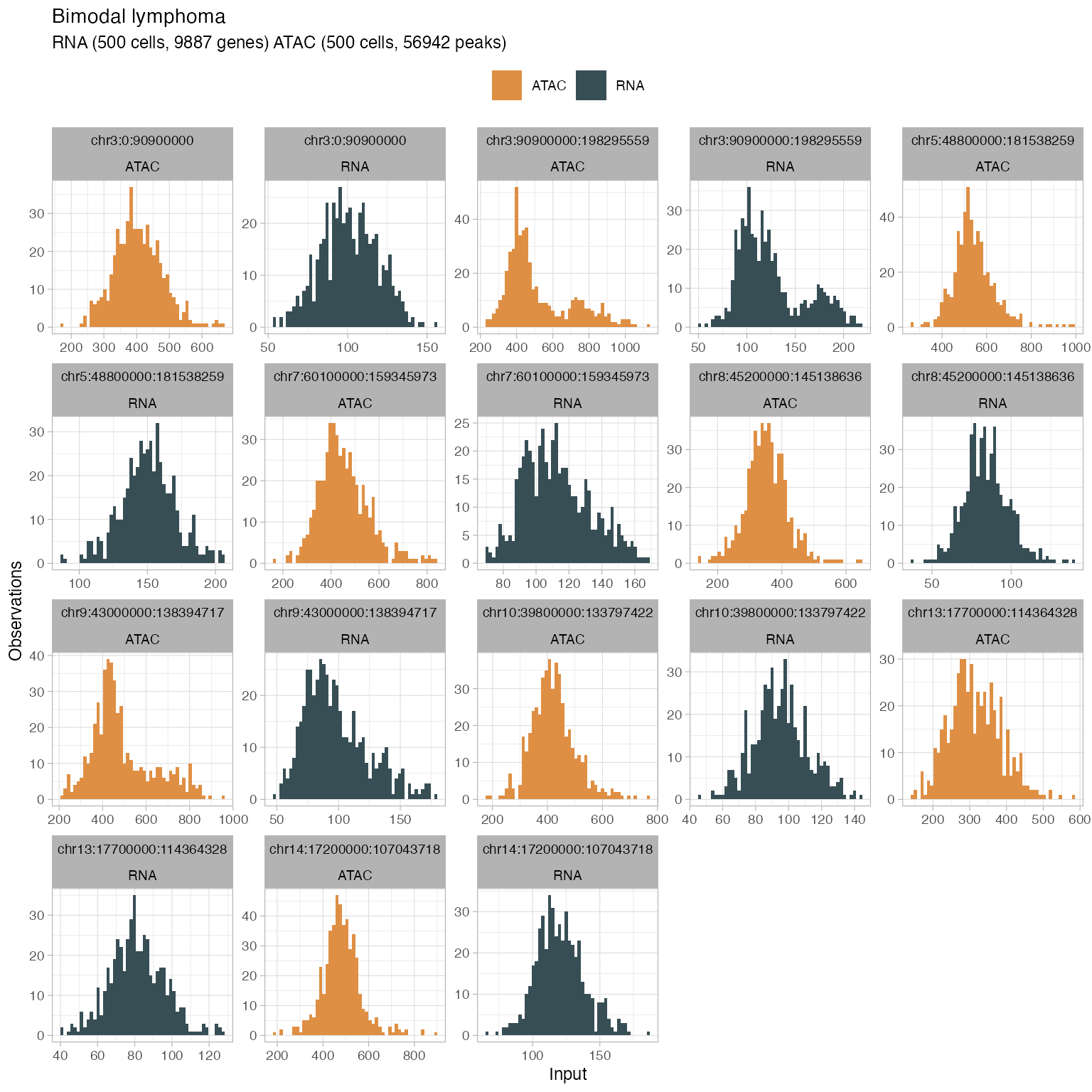
Add metadata to annotate the counts distributions
data(metadata)

x$input$metadata = metadata

plot_data(x,
  to_plot = 'type',
  position = 'stack',
  segments = get_input(x, what = 'segmentation') %>%
    ungroup() %>%
    mutate(L = to - from) %>%
    dplyr::arrange(dplyr::desc(L)) %>%
    dplyr::top_n(9) %>%
    pull(segment_id))
#> → Normalising RNA counts using input normalisation factors.
#> → Normalising ATAC counts using input normalisation factors.
#> Selecting by L
#> → Showing all segments (this plot can be large).
#> Joining with `by = join_by(cell)`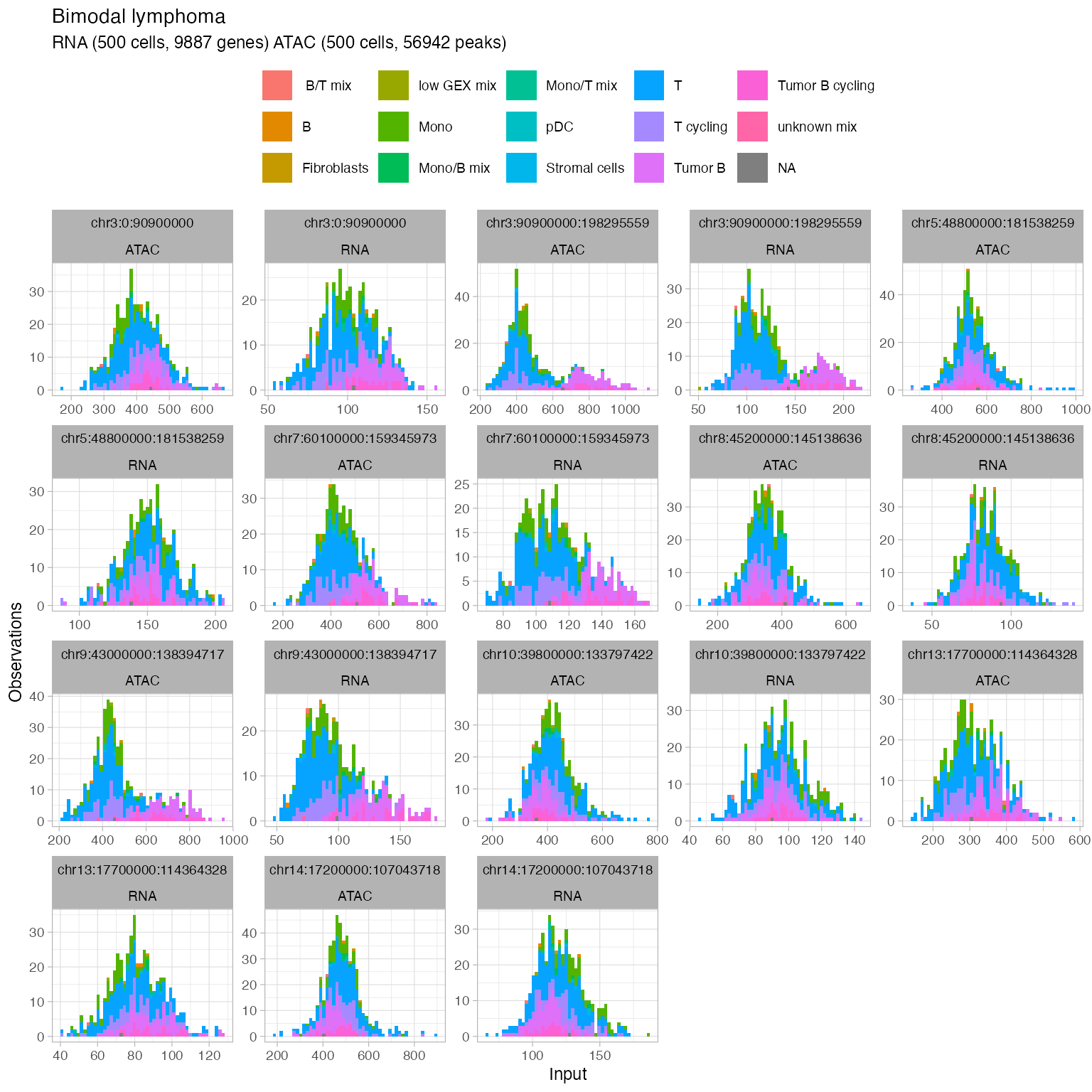
Please see the next vignette that shows how to perform CONGAS+ inference.