Setup the directory where results are stored.
sample = 'lymphoma'

prefix = paste0(sample, "/tutorial/")

out.dir = paste0(prefix, "/congas_data/")
fig.dir = paste0(prefix, "/congas_figures/")

if (!dir.exists(out.dir)) {dir.create(out.dir, recursive = T)}
if (!dir.exists(fig.dir)) {dir.create(fig.dir, recursive = T)}
We load the object created in the previous Vignette .
data(multiome_congas_object) To reduce the paramter search space dimensions and subsequently decreasing the computational complecity of CONGAS+ inference, users can optionally decide to perform a preliminary step of segment filtering, which consists in running CONGAS+ inference independently on each segment, varying the number of clusters from 1 to 3 and finally keeping only those segments in which the otpimal number of clusters selected by BIC is higher than 1.
This step is implemented in the fuction
segments_selector_congas, which return the filtered CONGAS+
object.
Fitting uses reticulate to interface with the Python
CONGAS package, which implements the models in Pyro. In case R does not
find a anaconda environment with CONGAS+ python version installed, it
will automatically create a r-reticulate environment and install CONGAS+
within that environment.
filt = segments_selector_congas(multiome_congas_object)
#> Warning: replacing previous import 'cli::num_ansi_colors' by
#> 'crayon::num_ansi_colors' when loading 'easypar'
# You can save the filtering result to avoid re-running the whole pipeline in future steps
# saveRDS(filt, paste0(out.dir, "rcongas_obj_filtered.rds"))
Now we can run CONGAS+ parameters inference on the final filtered object. We first using , and then we fit the model. The function computes the hyperparameters values using the current data. Its parameter is used to specify if the data contains a subset of normal cells. In case this is set to , the copy number distribution for one of the clusters will be initialized with values skewed towards the diploid state in every segment.
# Set values fro the model hyperparameters
k = c(1:4)

binom_limits = c(40,1000)
model = "BIC"

lr = 0.01
temperature = 20

steps = 5000
lambda = 0.5

# Estimate hyperparameters
hyperparams_filt <- auto_config_run(filt, k,
                                    prior_cn=c(0.2, 0.6, 0.1, 0.05, 0.05),
                                    init_importance = 0.6,
                                    CUDA = FALSE,
                                    normal_cells=TRUE)
#> ── (R)CONGAS+ hyperparameters auto-config ──────────────────────────────────────
#>
#> ── ATAC modality ──
#>
#> → Negative Binomial likelihood, estimating Gamma shape and rate
#>
#> ── Estimating segment factors
#> → 1: chr18:0:18500000 theta_shape = 9.19898572042463, theta_rate = 0.134656196154735
#> → 2: chr18:18500000:80373285 theta_shape = 9.79787953384757, theta_rate = 0.0438621501984607
#> → 3: chr3:90900000:198295559 theta_shape = 9.17167289102108, theta_rate = 0.0155177176789159
#> → 4: chr7:0:60100000 theta_shape = 11.9716723078498, theta_rate = 0.0335830102341236
#> → 5: chr9:43000000:138394717 theta_shape = 12.6405354431144, theta_rate = 0.022602435565188
#>
#> ── RNA modality ──
#>
#> → Negative Binomial likelihood, estimating Gamma shape and rate
#>
#> ── Estimating segment factors
#> → 1: chr18:0:18500000 theta_shape = 5.11720455085432, theta_rate = 0.31999035300107
#> → 2: chr18:18500000:80373285 theta_shape = 13.5825852942828, theta_rate = 0.240347578487164
#> → 3: chr3:90900000:198295559 theta_shape = 14.326975650189, theta_rate = 0.0910771911618621
#> → 4: chr7:0:60100000 theta_shape = 13.1313284095014, theta_rate = 0.148145381976511
#> → 5: chr9:43000000:138394717 theta_shape = 15.3629122806536, theta_rate = 0.124101739386109

# Run
hyperparams_filt$binom_prior_limits = binom_limits

fit_filt <- Rcongas:::fit_congas(filt,
                                 K = k,
                                 lambdas = lambda,
                                 learning_rate = lr,
                                 steps = steps,
                                 model_parameters = hyperparams_filt,
                                 model_selection = model,
                                 latent_variables = "G",
                                 CUDA = FALSE,
                                 temperature = temperature,
                                 same_mixing = TRUE,
                                 threshold = 0.001)
#> ✖ Warning ATAC 0-counts cells. 2 cells have no data in any of 5 segments, top 2 with missing data are:
#> ✖ Cell GTCCTAGAGCCAAATC-1-ATAC with 1 0-segments (20%)
#> ✖ Cell TCTCGCCCAAACATAG-1-ATAC with 1 0-segments (20%)
#>
#> ──  (R)CONGAS+  Variational Inference ──────────────────────────────────────────
#>
#> ── Fit with k = 1 and lambda = 0.5.
#>
#> Done!
#>
#> Computing assignment probabilities
#> Computing information criteria.
#>
#> ── Fit with k = 2 and lambda = 0.5.
#>
#> Done!
#>
#> Computing assignment probabilities
#> Computing information criteria.
#>
#> ── Fit with k = 3 and lambda = 0.5.
#>
#> Done!
#>
#> Computing assignment probabilities
#> Computing information criteria.
#>
#> ── Fit with k = 4 and lambda = 0.5.
#>
#> Done!
#>
#> Computing assignment probabilities
#> Computing information criteria.
#>
#> ── (R)CONGAS+ fits completed in 2m 57s. ──
#>
#> Joining with `by = join_by(cell)`
#> Joining with `by = join_by(cell)`
#> ✖ Warning ATAC 0-counts cells. 2 cells have no data in any of 5 segments, top 2 with missing data are:
#> ✖ Cell GTCCTAGAGCCAAATC-1-ATAC with 1 0-segments (20%)
#> ✖ Cell TCTCGCCCAAACATAG-1-ATAC with 1 0-segments (20%)
#> ── [ (R)CONGAS+ ] Bimodal lymphoma ─────────────────────────────────────────────
#>
#> ── CNA segments (reference: GRCh38)
#> → Input 5 CNA segments, mean ploidy 2.
#>
#>    | | |
#>
#>   Ploidy:    0     1     2     3     4     5     *
#>
#> ── Modalities
#> → RNA: 500 cells with 2034 mapped genes, 107643 non-zero values. Likelihood: Negative Binomial.
#> → ATAC: 500 cells with 15023 mapped peaks, 384290 non-zero values. Likelihood: Negative Binomial.
#>
#> ── Clusters: k = 2, lambda: l = 0.5, model with BIC = 22568.55.
#>
#>    C1     | | |
#>    C2     | | |
#>
#>     RNA
#>   C1 :  ■■■■■■ n = 124
#>   C2 :  ■■■■■■■■■■■■■■■■■■■ n = 376
#>     ATAC
#>   C1 :  ■■■■■■ n = 124
#>   C2 :  ■■■■■■■■■■■■■■■■■■■ n = 376
#>
#> ──  LOG  ──
#> - 2024-04-03 17:06:34.686264 Created input object.
#> - 2024-04-03 17:06:38.989073 Filtered s123egments: [0|50|50]
The new object has more information.
fit_filt
#> ✖ Warning ATAC 0-counts cells. 2 cells have no data in any of 5 segments, top 2 with missing data are:
#> ✖ Cell GTCCTAGAGCCAAATC-1-ATAC with 1 0-segments (20%)
#> ✖ Cell TCTCGCCCAAACATAG-1-ATAC with 1 0-segments (20%)
#> ── [ (R)CONGAS+ ] Bimodal lymphoma ─────────────────────────────────────────────
#>
#> ── CNA segments (reference: GRCh38)
#> → Input 5 CNA segments, mean ploidy 2.
#>
#>    | | |
#>
#>   Ploidy:    0     1     2     3     4     5     *
#>
#> ── Modalities
#> → RNA: 500 cells with 2034 mapped genes, 107643 non-zero values. Likelihood: Negative Binomial.
#> → ATAC: 500 cells with 15023 mapped peaks, 384290 non-zero values. Likelihood: Negative Binomial.
#>
#> ── Clusters: k = 2, lambda: l = 0.5, model with BIC = 22568.55.
#>
#>    C1     | | |
#>    C2     | | |
#>
#>     RNA
#>   C1 :  ■■■■■■ n = 124
#>   C2 :  ■■■■■■■■■■■■■■■■■■■ n = 376
#>     ATAC
#>   C1 :  ■■■■■■ n = 124
#>   C2 :  ■■■■■■■■■■■■■■■■■■■ n = 376
#>
#> ──  LOG  ──
#>
#> - 2024-04-03 17:06:34.686264 Created input object.
#> - 2024-04-03 17:06:38.989073 Filtered s123egments: [0|50|50]
You can get the information regarding model selection metrics
fit_filt$model_selection
#> # A tibble: 4 × 14
#>      NLL    AIC    BIC    ICL  entropy NLL_rna NLL_atac n_params n_observations
#>    <dbl>  <dbl>  <dbl>  <dbl>    <dbl>   <dbl>    <dbl>    <dbl>          <int>
#> 1 12180. 24452. 24677. 24677.  5.00e-8   9917.   14443.       46           1000
#> 2 11036. 22215. 22569. 22578. -9.27e+0   9228.   12843.       72           1000
#> 3 11005. 22207. 22688. 22864. -1.76e+2   9191.   12820.       98           1000
#> 4 11005. 22258. 22867. 23042. -1.76e+2   9192.   12818.      124           1000
#> # ℹ 5 more variables: hyperparameter_K <int>, K <int>, K_rna <int>,
#> #   K_atac <int>, lambda <dbl>
Rcongas::plot_fit(fit_filt, what='scores')
plot_fit(fit_filt, 'posterior_CNA')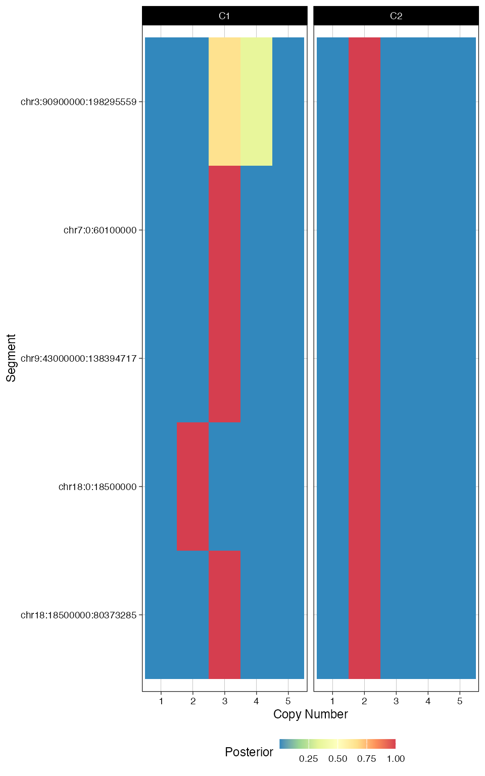
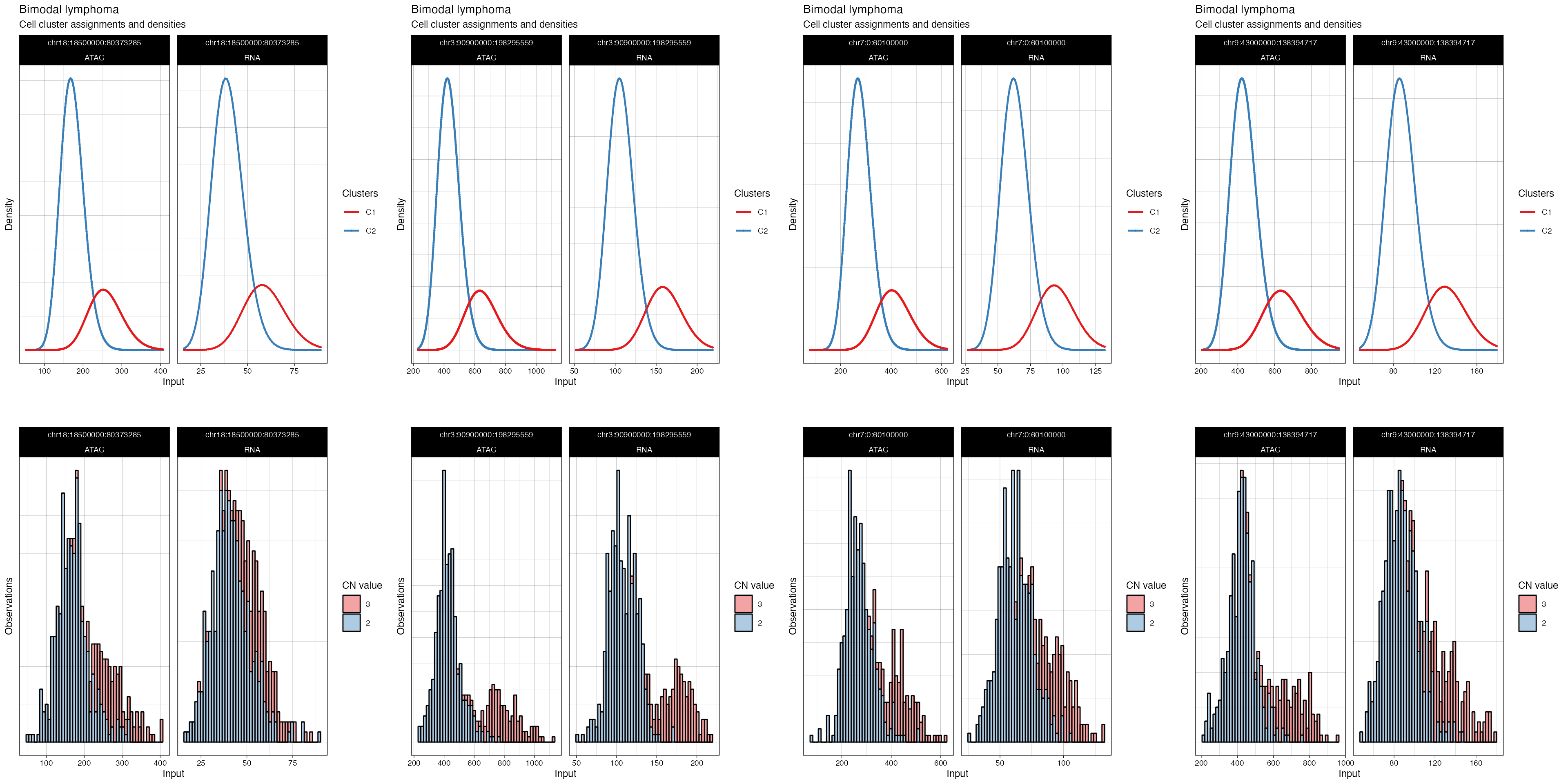
p = cowplot::plot_grid(
  plotlist = plot_fit(fit_filt, what = 'density', highlights = TRUE),
  ncol = 4)
#> → Plotting segments where different CNAs are present: chr18:18500000:80373285, chr3:90900000:198295559, chr7:0:60100000, and chr9:43000000:138394717.
#> → Normalising RNA counts using input normalisation factors.
#> → Normalising ATAC counts using input normalisation factors.
#> → Showing all segments (this plot can be large).
#> Joining with `by = join_by(cell)`
#> → Normalising ATAC counts using input normalisation factors.
#> → Normalising RNA counts using input normalisation factors.
#> Joining with `by = join_by(cluster, modality)`
#> Joining with `by = join_by(segment_id, cluster)`
#> Warning: The `<scale>` argument of `guides()` cannot be `FALSE`. Use "none" instead as
#> of ggplot2 3.3.4.
#> ℹ The deprecated feature was likely used in the Rcongas package.
#>   Please report the issue to the authors.
#> This warning is displayed once every 8 hours.
#> Call `lifecycle::last_lifecycle_warnings()` to see where this warning was
#> generated.
p