3. Inferring uknwokn breakpoints • biPOD

library(biPOD)
require(dplyr)
#> Loading required package: dplyr
#> 
#> Attaching package: 'dplyr'
#> The following objects are masked from 'package:stats':
#> 
#>     filter, lag
#> The following objects are masked from 'package:base':
#> 
#>     intersect, setdiff, setequal, union

In the previous task we assumed that the break points, i.e. the instant of time in which the latent dynamics changes abruptly, were know a priori. However, this is often not the case and one might be interested in inferring them.

Input data

We take the xenografts data and we make it ready for inference by preparing the count column and by dividing the time column by a factor of 7 (in order to work with a unit of time of a week).

We select the sample 543, already presented in the previous vignette.

data("xenografts", package = "biPOD")
mouse_id <- 543
d <- xenografts %>%
  dplyr::rename(count = tumour_volume) %>%
  dplyr::mutate(time = time / 7) %>%
  dplyr::filter(mouse == mouse_id)

Breakpoints inference

You can infer the breakpoints in the following way. After having initialized a bipod object with no breakpoints you can use the function fit_breakpoints.

If you reasonably know the possible number of breakpoints, you should pass a vector to the available_changepoints.

x <- biPOD::init(d, sample = mouse_id, break_points = NULL)
#> 
#> ── biPOD - bayesian inference for Population Dynamics ──────────────────────────
#> ℹ Using sample named: 543.
#> ! No group column present in input dataframe! A column will be added.
biPOD::plot_input(x)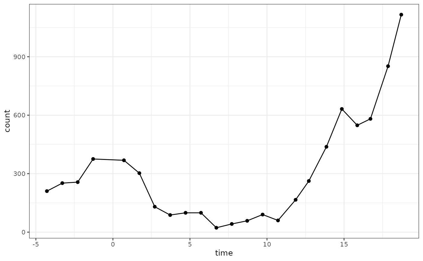

x <- biPOD::fit_breakpoints(x, norm = T, n_trials = 500, avg_points_per_window = 3, available_changepoints = c(0,2), model_selection = "LOO", n_core=1)
#> ℹ Intializing breakpoints...
#> ℹ Breakpoints optimization...
#> ℹ Choosing optimal breakpoints...
#> ℹ Median of the inferred breakpoints have been succesfully stored.
x
#> ── [ biPOD ] 23 observations divided in 3 time windows. ────────────────────────
#> 
#> ── Break-points inference  PASS  Mean rhat = 1. ────────────────────────────────
#> ℹ  Number of breakpoints inferred : 2
#> # A tibble: 2 × 7
#>   Parameter  Mean    Sd   p05   p50   p95  Rhat
#>   <chr>     <dbl> <dbl> <dbl> <dbl> <dbl> <dbl>
#> 1 b[1]      0.143 0.705 -1.02 0.143  1.29  1.00
#> 2 b[2]      6.90  0.705  5.77 6.87   8.11  1.00

The inferred breakpoints are now stored in the metadata$breakpoints field.

print(x$metadata$breakpoints)
#> [1] 0.142927 6.874915

and their posterior distribution can be visualized using plot_breakpoints_posterior function

biPOD::plot_breakpoints_posterior(x)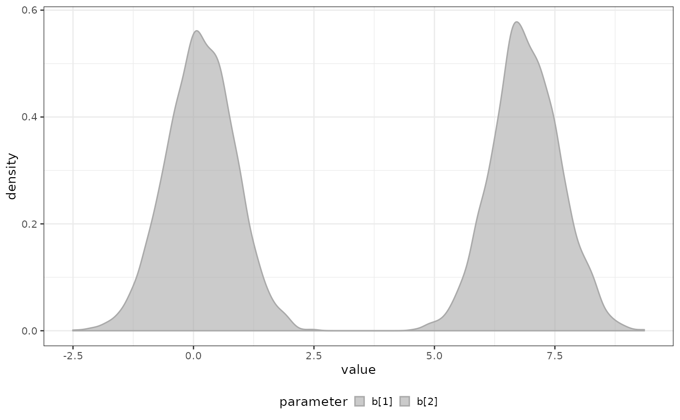

Re-fit task 1

Now that the breakpoints have been inferred one can fit the data according to the first task simply using the fit function. Let’s see how it works on one example.

x <- biPOD::fit(
  x,
  growth_type = "both",
  infer_t0 = F
)
#> ℹ Fitting with model selection.
#> ℹ Model selection finished!
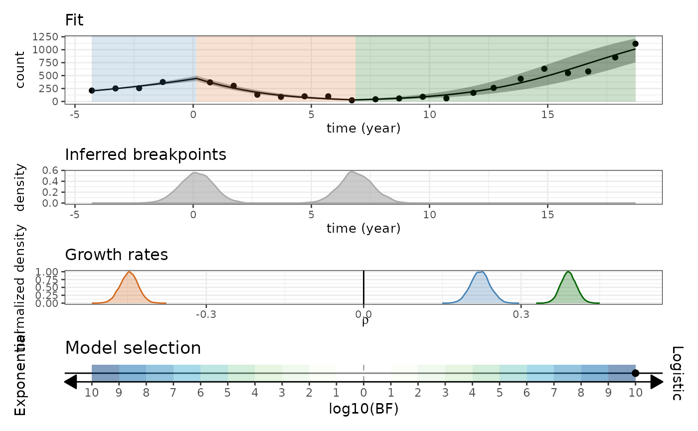
#> ℹ Model with "Logistic" growth deemed better with "Decisive" evidence. (BF = 847443020960387712)

And let’s look at the final result.

biPOD::plot_report(x, fit_type = 'simple')
#> ℹ Creating report...
#> ℹ Preparing fit plot...
#> ℹ Preparing breakpoints posterior plot...
#> ℹ Preparing growth rates posterior plot...
#> ℹ Preparing model selection plot...