2. Fitting dynamics with known breakpoints • biPOD

library(biPOD)
require(dplyr)
#> Loading required package: dplyr
#> 
#> Attaching package: 'dplyr'
#> The following objects are masked from 'package:stats':
#> 
#>     filter, lag
#> The following objects are masked from 'package:base':
#> 
#>     intersect, setdiff, setequal, union

The problem of characterizing a tumor growth model when growth rates change at known time-points while considering both exponential and logistic growths can be tackled using biPOD. In this vignette we are going to look at how to use biPOD for this specific problem.

Input data

We take the xenografts data and we make it ready for inference by preparing the count column and by dividing the time column by a factor of 7 (in order to work with a unit of time of a week).

data("xenografts", package = "biPOD")
xenografts <- xenografts %>%
  dplyr::rename(count = tumour_volume) %>%
  dplyr::mutate(time = time / 7)

Fit - Variational and no breakpoints

Let’s take a sample which does not undergo treatment and should therefore exhibit a natural growth with a single parameter. Hence, we are not going to consider any breakpoints for this sample.

mouse_id <- 537
d <- xenografts %>% dplyr::filter(mouse == mouse_id)
x <- biPOD::init(
  counts = d,
  sample = mouse_id,
  break_points = NULL
)
#> 
#> ── biPOD - bayesian inference for Population Dynamics ──────────────────────────
#> ℹ Using sample named: 537.
#> ! No group column present in input dataframe! A column will be added.

Once the bipod object has been initialized it is possible to visualize the data using the plot_input function.

biPOD::plot_input(x, log_scale = F, add_highlights = T)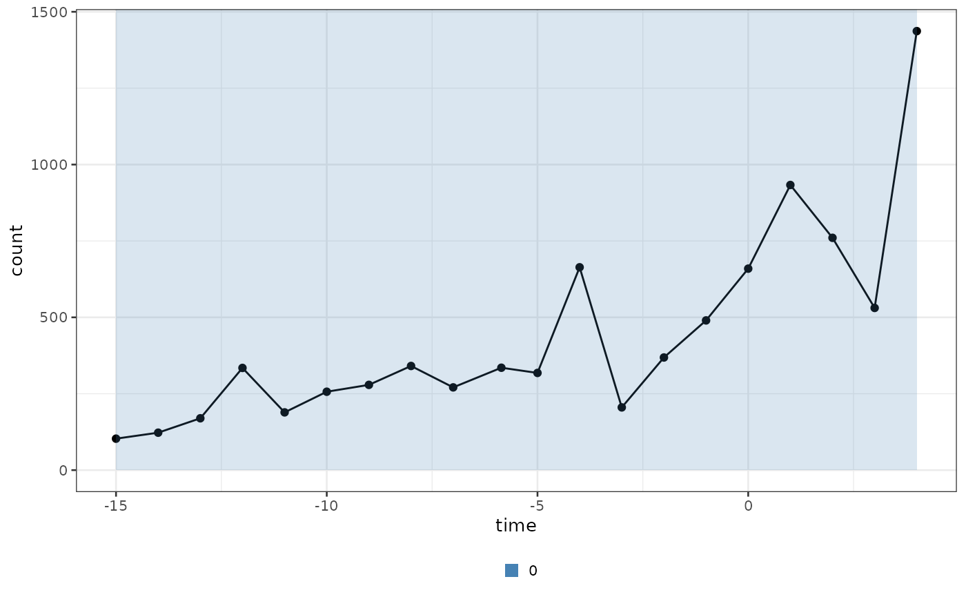

Now, to fit the data for the first task one has to use the fit function.

If you want to fit one specific type of growth (exponential or logistic) you have to pass one of the two to the parameter growth_type. Otherwise, if you want to test both of them and choose the best one you have to set the growth_type parameter to both.

Sometimes it might be helpful to scale the input data by a factor_size, so that all the counts will be divided by it.

When a population is decreasing or growing extremely slowly ( $\rho \sim 0$ ) the instant of time in which the population was born might be impossible to infer. To deal with such situations, or when $t_0$ is of no interest, just set the infer_t0 parameter to FALSE.

In order to use a Variational Inference algorithm it suffice to set the variational parameter to TRUE.

x <- biPOD::fit(
  x,
  growth_type = "both",
  model_selection_algo = "mixture_model",
  factor_size = 1,
  variational = T
)
#> ℹ Fitting with model selection.
#> ! The first step of the inference will be performed using MCMC...

Plot - Variational and no breakpoints

Diagnostics

The first plot to look at would be the one regarding the diagnostic of the inference. In this case, having used VI, we are going to look at the ELBO. To do so, let’s use the plot_elbo function which requires a bipod object and the specification of which elbo data we want to use since there might be multiple if we perform different task on the same object.

biPOD::plot_elbo(x, elbo_data = x$fit_elbo, diagnose = T)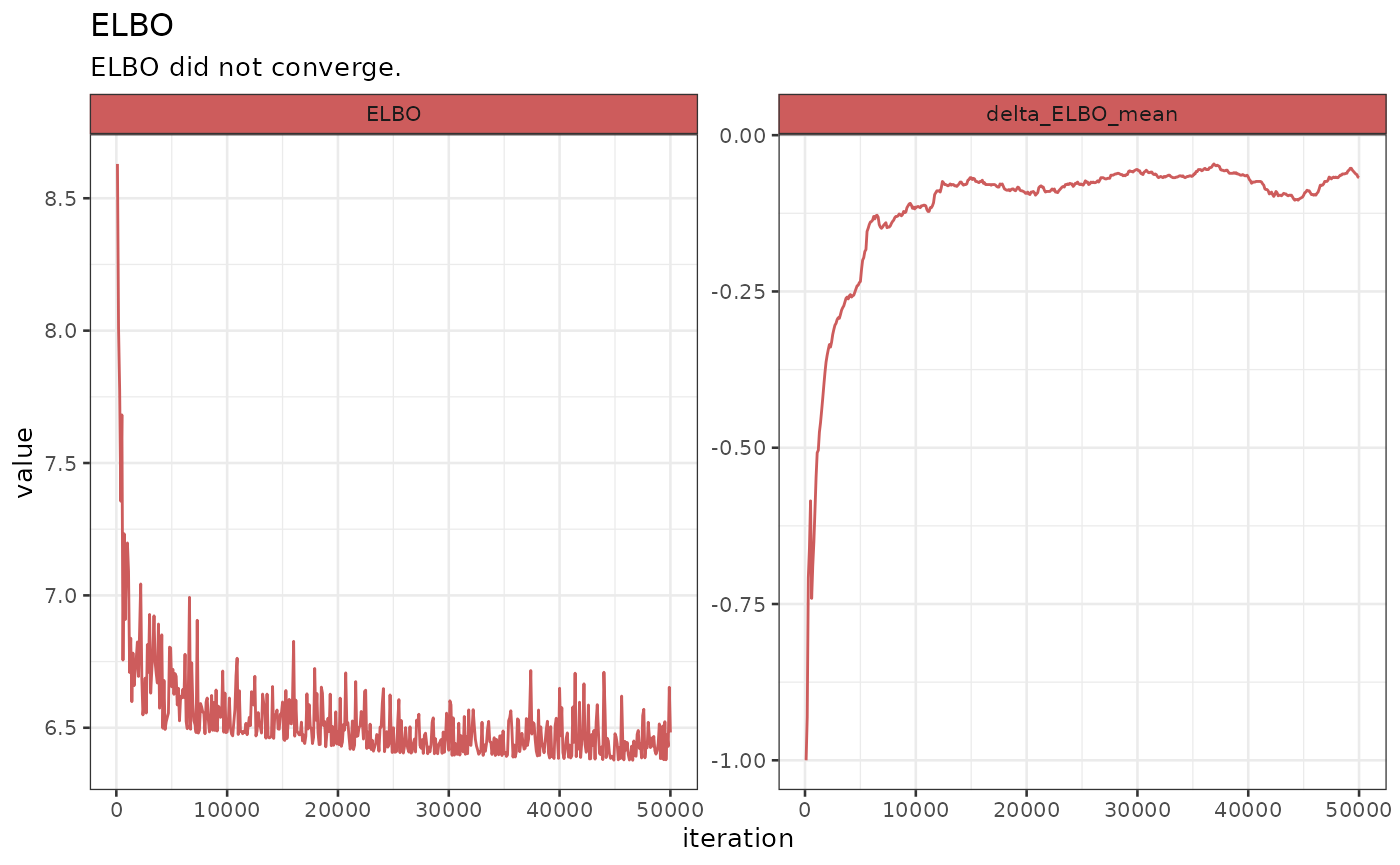

Plot of fit

Use the function plot_fit to plot the fit resulting after the inference of the first task.

Set zoom to TRUE to have a better view of the observations and full_process to TRUE to also plot the inferred value of $t_0$ .

biPOD::plot_fit(x = x, zoom = T, full_process = T)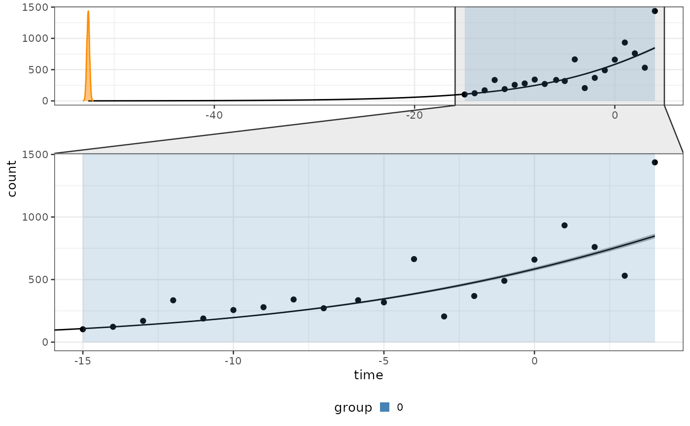

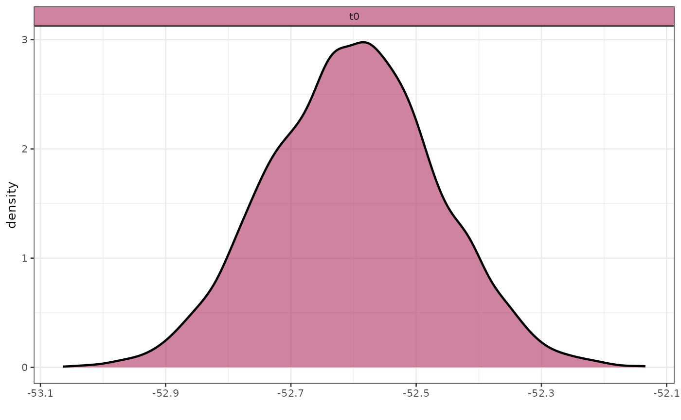
Plot posteriors

You can use the general function plot_posterior to plot the posterior for a given parameters (use plot_posteriors for a set of parameters).

The names of the available parameters can be found in one of the fit objects inside the bipod object. For example in this case let’s plot $t_0$ .

print(x$fit$parameters)
#>  [1] "lp__"        "lp_approx__" "rho[1]"      "t0"          "K"          
#>  [6] "log_lik[1]"  "log_lik[2]"  "log_lik[3]"  "log_lik[4]"  "log_lik[5]" 
#> [11] "log_lik[6]"  "log_lik[7]"  "log_lik[8]"  "log_lik[9]"  "log_lik[10]"
#> [16] "log_lik[11]" "log_lik[12]" "log_lik[13]" "log_lik[14]" "log_lik[15]"
#> [21] "log_lik[16]" "log_lik[17]" "log_lik[18]" "log_lik[19]" "log_lik[20]"
#> [26] "yrep[1]"     "yrep[2]"     "yrep[3]"     "yrep[4]"     "yrep[5]"    
#> [31] "yrep[6]"     "yrep[7]"     "yrep[8]"     "yrep[9]"     "yrep[10]"   
#> [36] "yrep[11]"    "yrep[12]"    "yrep[13]"    "yrep[14]"    "yrep[15]"   
#> [41] "yrep[16]"    "yrep[17]"    "yrep[18]"    "yrep[19]"    "yrep[20]"
biPOD::plot_posterior(
  x,
  x_fit = x$fit,
  par_name = "t0",
  color = "maroon"
)

Model selection

Since we selected between exponential and logistic there is also the possibility to visualize this decision. In this case, having used the mixture_model algorithm we can plot it using the ``

biPOD::plot_mixture_model_omega(x, plot_type = "boxplot", color = "forestgreen")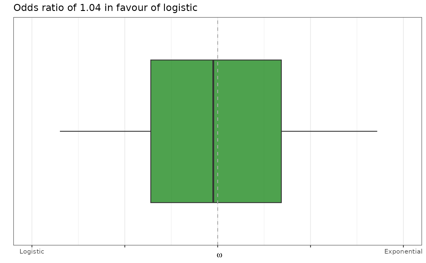

Fit - MCMC and with breakpoints

Let’s now consider a sample that undergoes treatment and should therefore exhibit a multiple growth rates. For this tutorial we will work with two manually chosen breakpoints (i.e 0 and 7).

mouse_id <- 543
d <- xenografts %>% dplyr::filter(mouse == mouse_id)
x <- biPOD::init(
  counts = d,
  sample = mouse_id,
  break_points = c(0, 7)
)
#> 
#> ── biPOD - bayesian inference for Population Dynamics ──────────────────────────
#> ℹ Using sample named: 543.
#> ! No group column present in input dataframe! A column will be added.

Now the input will be grouped in different time windows, as it can also be seen by plotting it.

biPOD::plot_input(x, log_scale = T, add_highlights = T)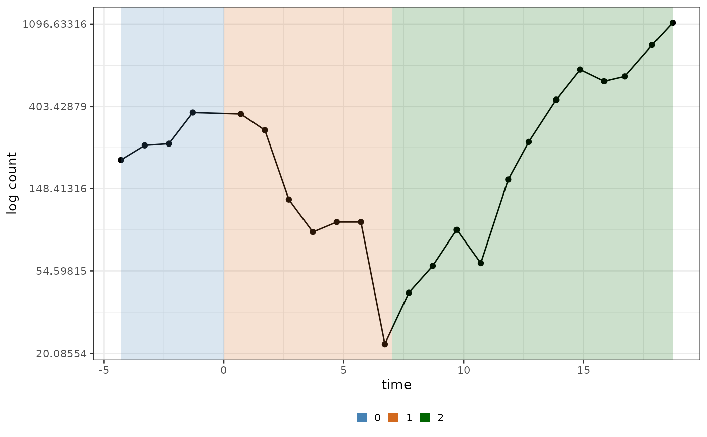

Let’s use again the fit function.

We want to use the MCMC algorithm so make sure to set the variational parameter to FALSE.

Moreover, we are going to use bayes_factor as a model selection algorithm.

x <- biPOD::fit(
  x,
  growth_type = "both",
  model_selection_algo = "bayes_factor",
  variational = FALSE
)

Plot - MCMC and with breakpoints

Diagnostics

Let’s plot the diagnostic of the inference. In this case, having used MCMC, we are going to look at the chains to see if they’ve mixed properly. To do so, let’s use the plot_traces function which requires a bipod object and the specification of which fit we want to use since there might be multiple if we perform different task on the same object.

biPOD::plot_traces(x, fit = x$fit, pars = NULL, diagnose = T)
#> ℹ The input vector 'pars' is empty. All the following parameters will be
#> reported: "lp__", "rho[1]", "rho[2]", "rho[3]", "t0", "K", "log_lik[1]",
#> "log_lik[2]", "log_lik[3]", "log_lik[4]", "log_lik[5]", "log_lik[6]",
#> "log_lik[7]", "log_lik[8]", "log_lik[9]", "log_lik[10]", "log_lik[11]",
#> "log_lik[12]", …, "yrep[22]", and "yrep[23]".  It might take some time...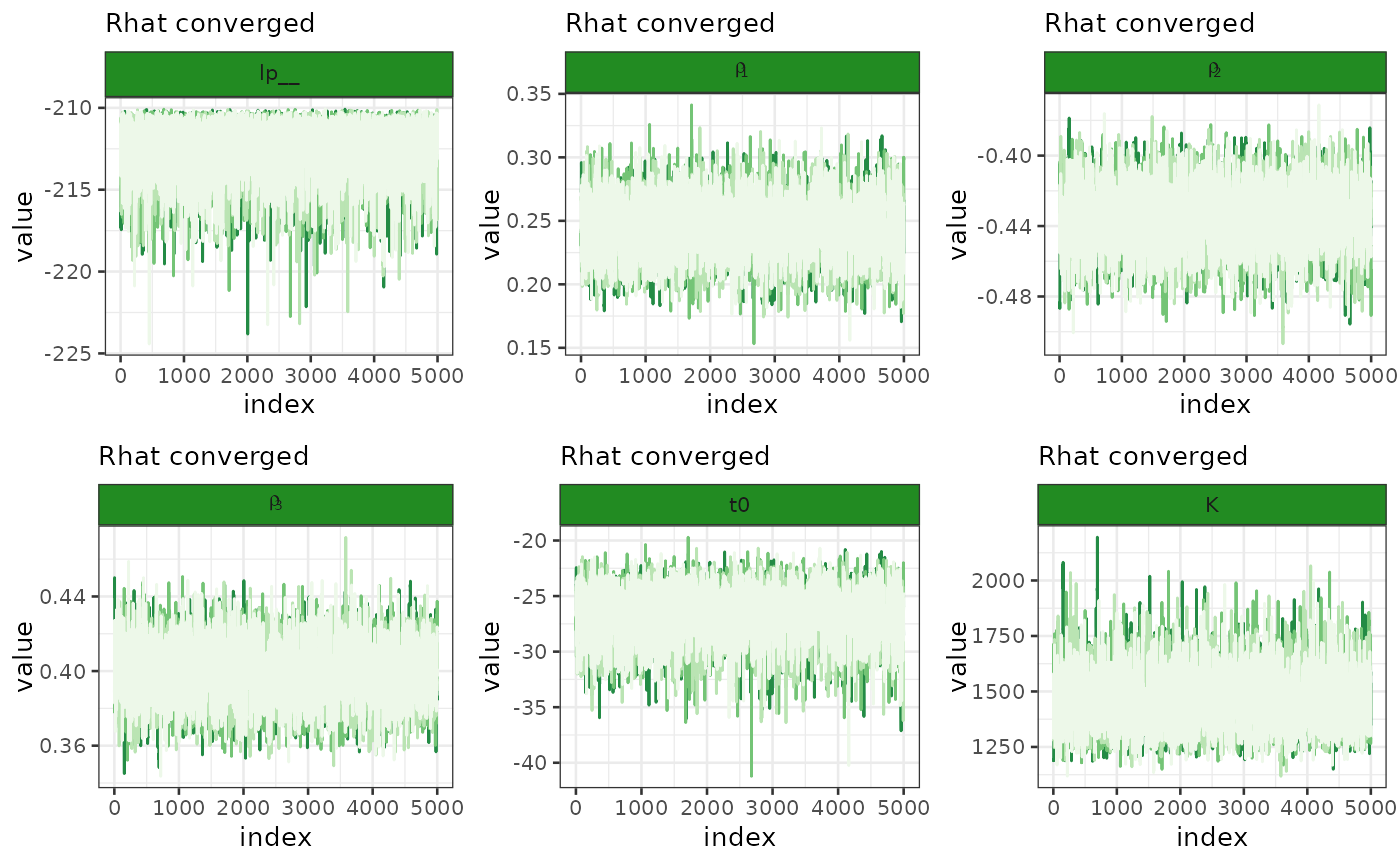

Plot of fit

Let’s use the function plot_fit. You can change the legend using the parameter legend_labels and legend_title.

biPOD::plot_fit(x = x, legend_labels = c("Natural growth", "Treatment", "Relapse"), legend_title = "Phase")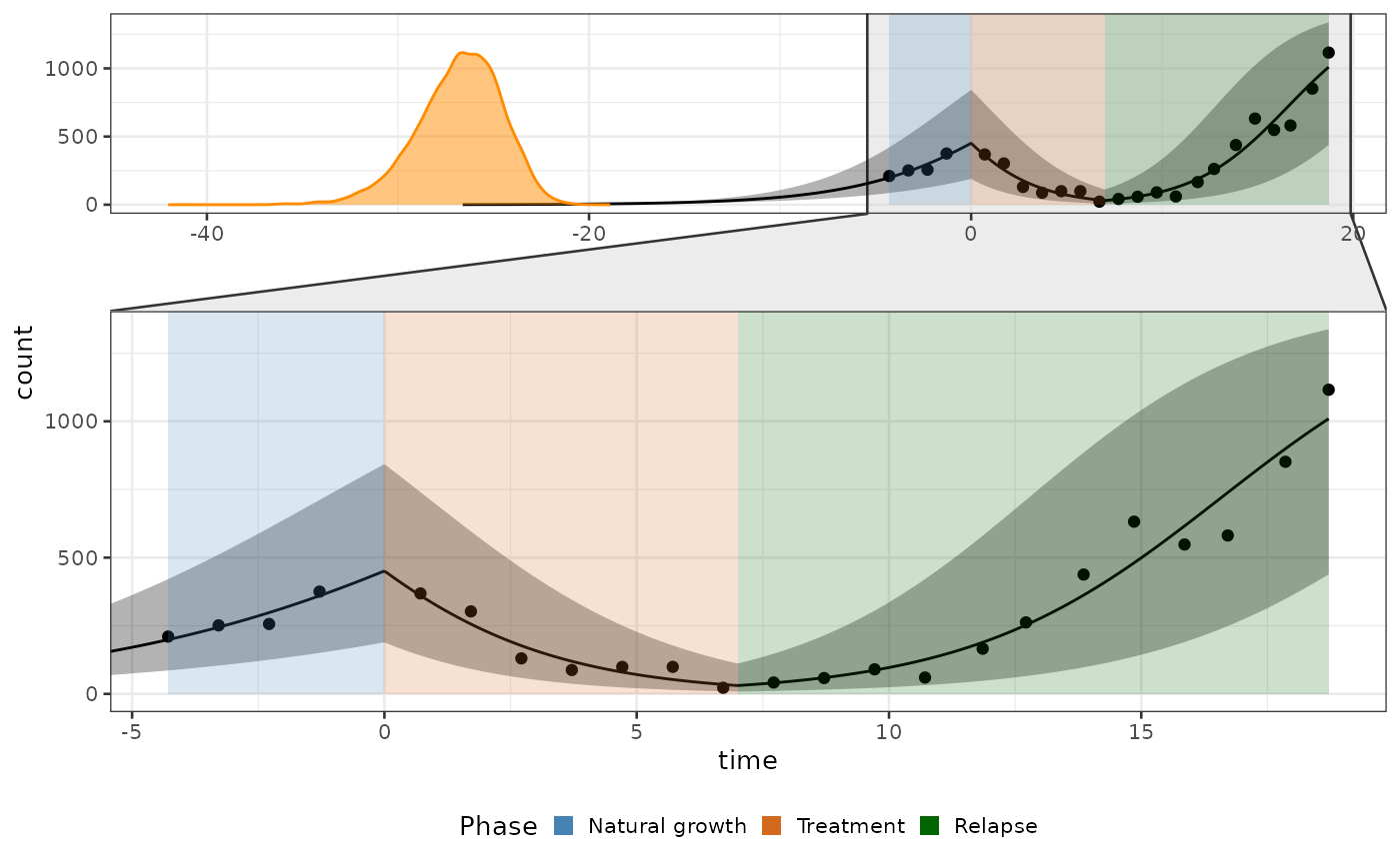

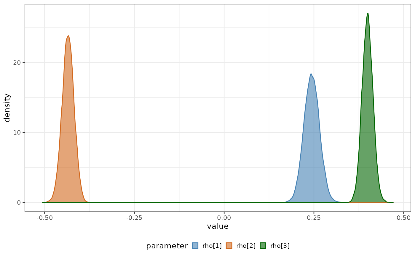
Plot of posteriors

Let’s use plot_posteriors function to plot all the growth rates one against each other.

biPOD::plot_posteriors(
  x,
  x_fit = x$fit,
  par_list = c("rho[1]", "rho[2]", "rho[3]")
)

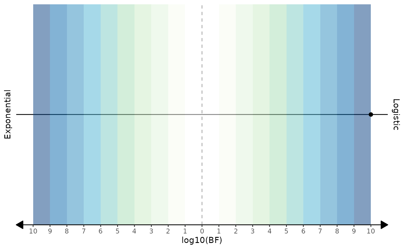
Model selection

And finally, let’s plot the Bayes factor using the plot_bayes_factor function.

biPOD::plot_bayes_factor(x, with_categories = F)