4. Fitting a mixture of resistant-sensitive population • biPOD

library(biPOD)
require(dplyr)
#> Loading required package: dplyr
#> 
#> Attaching package: 'dplyr'
#> The following objects are masked from 'package:stats':
#> 
#>     filter, lag
#> The following objects are masked from 'package:base':
#> 
#>     intersect, setdiff, setequal, union

When a population shrinks (e.g., sensitive to treatment) and later regrows (e.g., resistant to treatment) the dynamics are U-shaped. Here we are going to consider this specific case.

Input data

We take the xenografts data and we make it ready for inference by preparing the count column and by dividing the time column by a factor of 7 (in order to work with a unit of time of a week).

We select the sample 543, already presented in the previous vignette and we filter out the observations that are prior to the treatment.

data("xenografts", package = "biPOD")
mouse_id <- 543
d <- xenografts %>%
  dplyr::rename(count = tumour_volume) %>%
  dplyr::mutate(time = time / 7) %>%
  dplyr::filter(time >= 0) %>% 
  dplyr::filter(mouse == mouse_id)
x <- biPOD::init(d, "543 U-shape")
#> 
#> ── biPOD - bayesian inference for Population Dynamics ──────────────────────────
#> ℹ Using sample named: 543 U-shape.
#> ! No group column present in input dataframe! A column will be added.
biPOD::plot_input(x)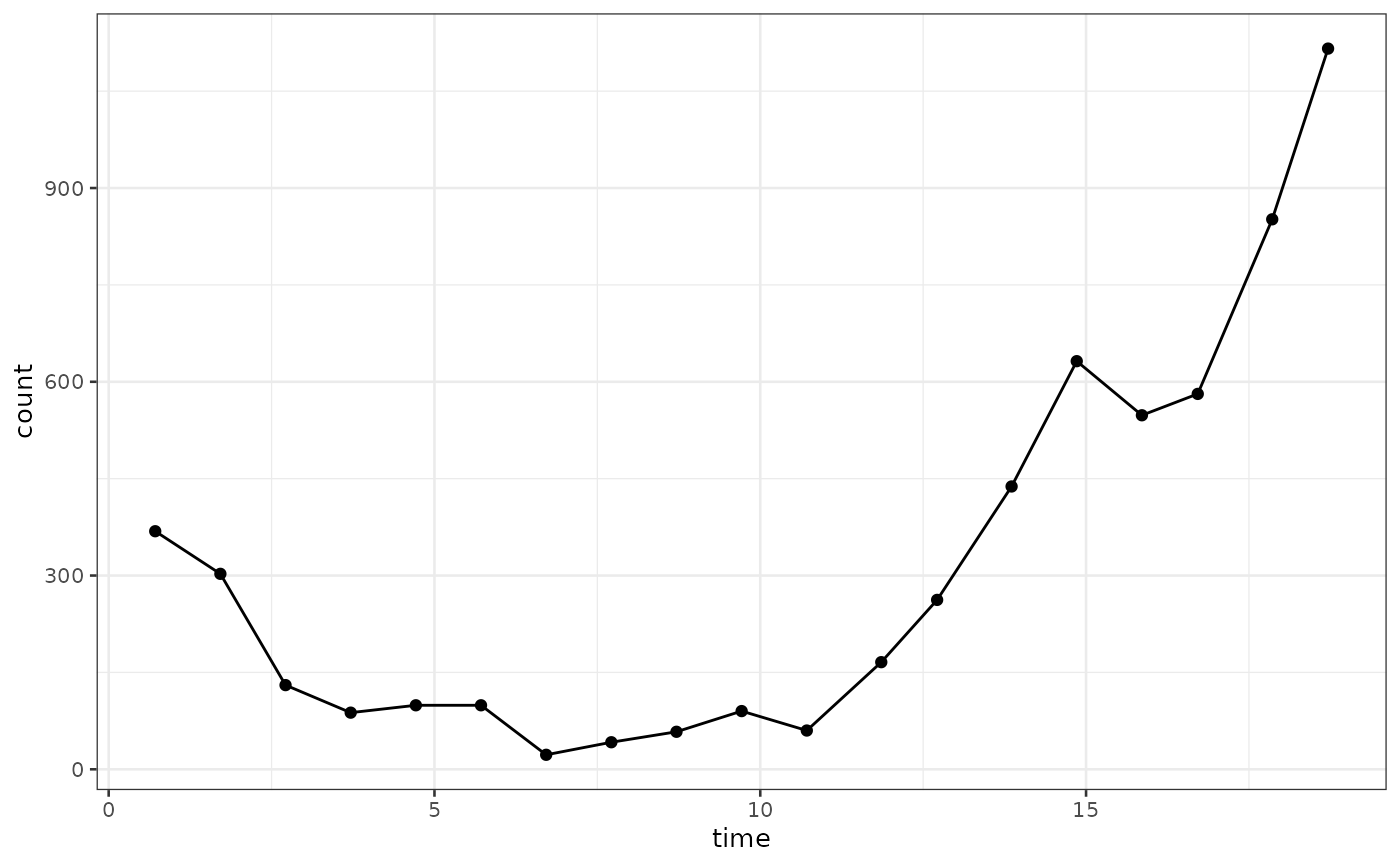

Two population model

The model assumes that

only two populations exist, one dying out and one growing
the growth rates are both positive and constant
the sensible population must be present at x=0 but the same does not apply for the resistant one

and is able to infer

$t_s$ , instant of time in which the sensitive population dies out
$t_r$ , instant of time in which the resistant population was born
$\rho_s$ , death rate of the sensitive population
$\rho_r$ , growth rate of the resistant population

To do so, one need to use the fit_two_pop_model function.

x <- biPOD::fit_two_pop_model(x, variational = F, factor_size = 1)
#> ℹ Fitting two population model using MCMC sampling ...
#> Warning: Some Pareto k diagnostic values are too high. See help('pareto-k-diagnostic') for details.
#> Warning: Some Pareto k diagnostic values are too high. See help('pareto-k-diagnostic') for details.
#> Warning: Dropping 'draws_df' class as required metadata was removed.
#> Warning: Dropping 'draws_df' class as required metadata was removed.
#> Warning: Dropping 'draws_df' class as required metadata was removed.
#> Warning: Dropping 'draws_df' class as required metadata was removed.
#> Warning: Dropping 'draws_df' class as required metadata was removed.
#> Warning: Dropping 'draws_df' class as required metadata was removed.
#> Warning: Dropping 'draws_df' class as required metadata was removed.

and the fit can be visualized as a single process

biPOD::plot_two_pop_fit(x, split_process = F, f_posteriors = F, t_posteriors = F, r_posteriors = F)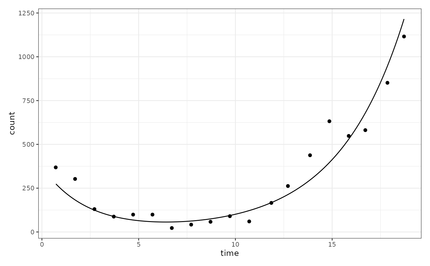

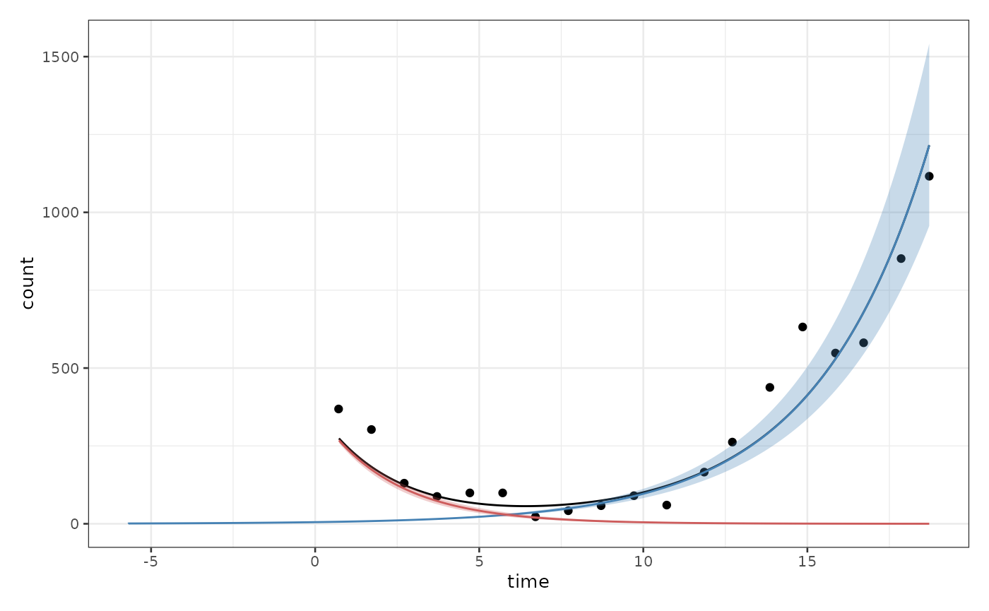
or splitting it depending on the two different populations

biPOD::plot_two_pop_fit(x, split_process = T, f_posteriors = F, t_posteriors = F, r_posteriors = F)