4. Visualising the results • TOSCA

See the Overview vignette for the core idea and a glossary of the terms used below.

Timing posteriors

The inferred timing posteriors can be visualised on the patient’s clinical timeline in two complementary ways: as histograms overlaid on a single timeline, or as stacked densities. In both plots, treatment periods are shown as coloured rectangles and sampling dates as points on the timeline.

TOSCA::plot_timing(UPN06)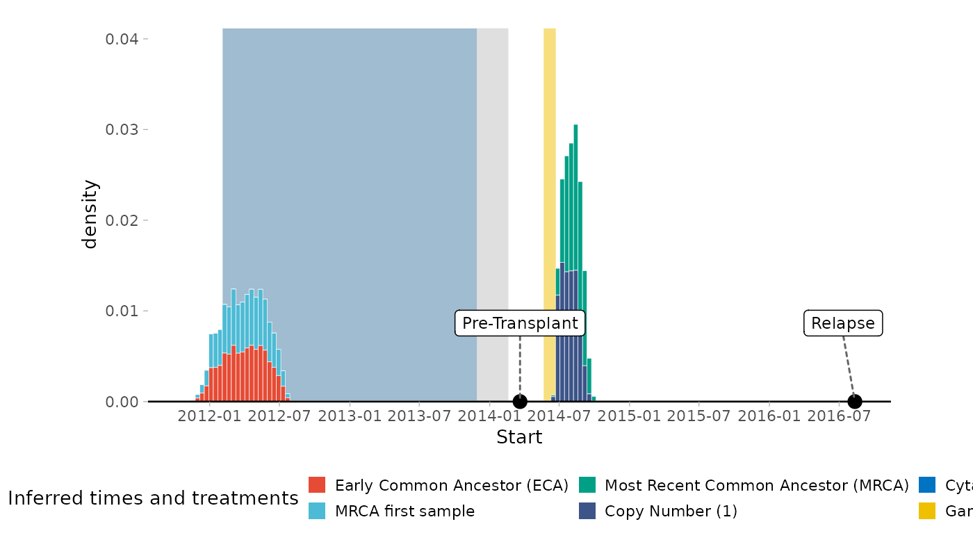

TOSCA::plot_timing_MAP(UPN06)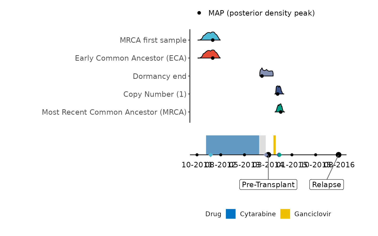

By default the x-axis is expressed in calendar dates. If preferred, timings can be displayed in days relative to a clinically meaningful reference event. For UPN06, we use the allo-HSCT date as the origin:

allo_HSCT <- "2014-04-23"
TOSCA::plot_timing_days(UPN06, days_from = allo_HSCT, event_name = "allo-HSCT")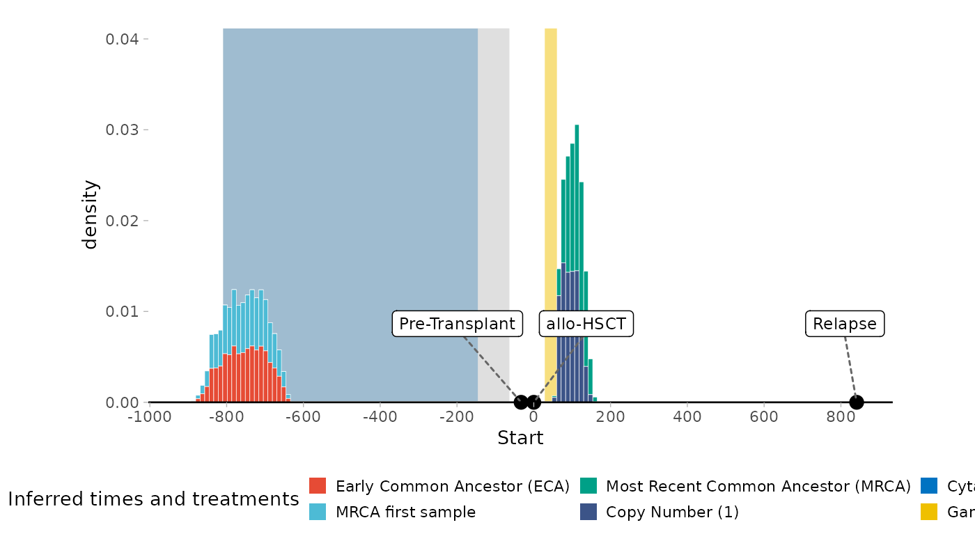

Summary statistics can likewise be computed relative to a reference date using days_from(). This is particularly useful for classifying the timed event as de novo (originating after the reference) or pre-existing (originating before it). For CNA-mediated resistance, the parameter t_cna and the length of the corresponding CNA, as specified in the mutations input, must be provided:

TOSCA::days_from(UPN06, from = allo_HSCT, parameter = "t_cna", cna_length = 47911693)
#> # A tibble: 1 × 4
#>   median  mean    q5      q95     
#>   <drtn>  <drtn>  <drtn>  <drtn>  
#> 1 95 days 96 days 65 days 132 days

Consistent with the findings reported in the companion clinical study, the posterior places the CNLOH of the HLA locus roughly 3 months after allo-HSCT, immediately following ganciclovir exposure, supporting a de novo origin of the resistance event rather than a pre-existing one. The same analysis estimated a tumour growth rate of $\omega \approx 10.9$ (a cell-doubling time of about 34 days) and a roughly 4.5-fold higher mutation rate during ganciclovir exposure compared to clock-like mutagenesis — both plausible for an actively expanding, drug-exposed clone, and a useful sanity check when interpreting your own fit() output against plot_prior_vs_posterior() below.

Dynamic parameters

To assess the inferred dynamic parameters, plot_prior_vs_posterior() displays the prior density alongside the posterior histogram for each parameter. The posterior median is indicated by a vertical red line.

TOSCA::plot_prior_vs_posterior(UPN06)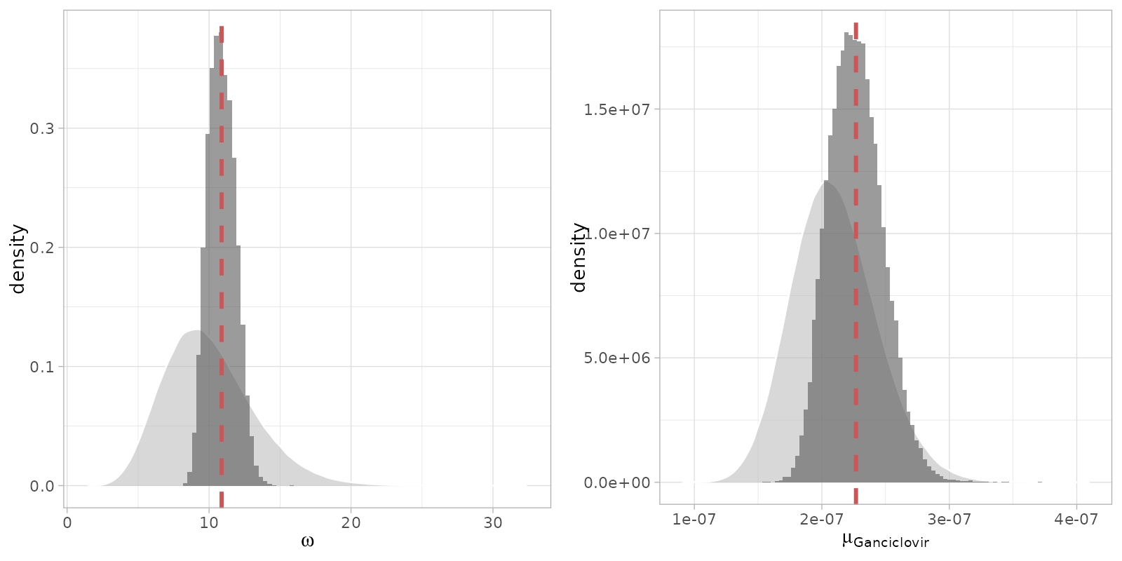

Posterior predictive check

To verify that the inferred parameters are compatible with the observed data, plot_ppc() displays the multivariate posterior predictive distribution (PPD) for each mutation group. The observed mutation count is shown as a red point; the PPD is represented as a cloud of draws, colour-coded by their distance from the observed value.

TOSCA::plot_ppc(UPN06)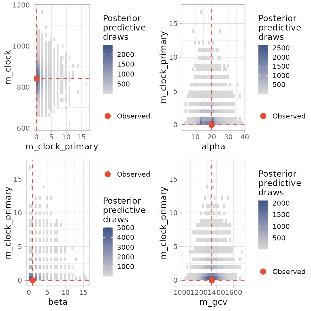

MCMC diagnostics

TOSCA exposes a suite of diagnostic plots built on the bayesplot package. These should be inspected routinely to verify that the sampler has explored the posterior adequately. Available diagnostics include chain trace plots, $\hat{R}$ plots, effective sample size (ESS) plots, and divergent transitions.

TOSCA::plot_mcmc_chains(UPN06)

TOSCA::rhats_plot(UPN06)

TOSCA::ess_plot(UPN06)

TOSCA::plot_divergent_transitions(UPN06)