2. Setting the priors • TOSCA

The TOSCA model

See the Overview vignette for the core idea and a glossary of the terms used below.

Intuition

Think of each mutational process (clock-like ageing, a mutagenic drug, a hypermutator driver) as a clock ticking at some rate, laying down mutations as it goes. Most of the time that rate is constant — but it can change: a drug’s clock only ticks while the drug is being administered, dormant cells stop ticking altogether, and a driver mutation can permanently speed a clock up. TOSCA counts how many “ticks” (mutations) landed in each category along the branch connecting the ECA to the MRCA, and works backwards to when each clock must have started or changed speed, given how fast it’s known (or assumed) to tick.

Formally, TOSCA models mutation accumulation as an inhomogeneous Poisson process whose rate varies over time according to the clinical history of the patient and the latent timing of clonal events. Mutations are partitioned into groups by mutational process and karyotype, and each group accumulates independently. For a group $s$ , the expected mutation count is:

$m_s \sim \text{Poisson}\left( n_s \cdot \ell_s \cdot \omega \cdot \int_{t_{\text{start}}}^{t_{\text{end}}} \mu_s \, dt \right)$

where $n_s$ is the number of alleles (e.g. 2 for diploid mutations), $\ell_s$ is the length of the genomic region over which mutations accumulate, $\mu_s$ is the mutation rate for group $s$ , and $\omega$ is the tumour growth rate. Parameter inference is performed via Markov Chain Monte Carlo (MCMC).

TOSCA infers two sets of latent quantities:

Timing parameters: the time of origin of the early common ancestor (ECA), the time of origin of the resistant clone, and the time of origin of the most recent common ancestor (MRCA).
Dynamic parameters: the tumour growth rate $\omega$ and the mutation rate(s) $\mu_s$ under each therapy.

Two ways to time the resistant clone

The resistant clone’s origin can leave two different kinds of trace on the genome, and TOSCA reads whichever one applies (set via model_name when calling fit(), see the next vignette).

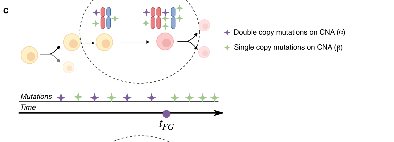
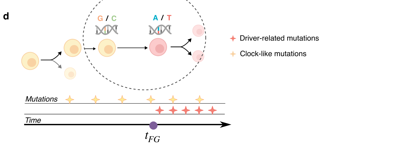
Left (model_name = "CNA"): a copy-number event doubles some mutations onto the new copy. The ratio of double-copy ( $\alpha$ ) to single-copy ( $\beta$ ) mutations positions the event in time — early events have more time to accumulate $\alpha$ mutations, late events almost none. Right (model_name = "Driver"): a driver mutation shifts the mutation rate and/or spectrum. The ratio of clock-like to driver-associated mutations plays the same role $\alpha/\beta$ plays for copy number. Figures adapted from the TOSCA manuscript (in preparation).

This shows up directly in the shape of the Mutations table. UPN06 (used throughout this series) is a CNA case — its private mutations include alpha/beta rows (see vignette 1). The toy dataset below, exampleData_Driver, illustrates the driver case instead: no CNA rows, but a driver mutation type carrying the count of driver-associated mutations accumulated after the shift.

library(TOSCA)
data("exampleData_Driver")
exampleData_Driver$Input$Mutations
#>           Name Length Karyotype               Type Value
#> 1 sbs1_primary  3e+09       1:1 clock-like primary   0.9
#> 2 sbs1_relapse  3e+09       1:1 clock-like relapse  78.0
#> 3        sbs11  3e+09       1:1             driver 150.0

We’ll fit this exact toy dataset live in the next vignette.

Setting the priors

The hyperparameters required to run TOSCA fall into three groups.

Timing parameters

The priors on the ECA, MRCA, and resistant clone origin times are set automatically as uniform distributions, with bounds derived from the clinical history provided at initialisation. Ordering constraints between events are enforced by construction (e.g. the ECA must precede the MRCA), and the clinical information further restricts the admissible intervals: for instance, if a therapy-associated mutational process is detected, TOSCA assumes that the MRCA originated no earlier than the start of the corresponding treatment. No user input is required for these priors.

Clock-like mutation rate

The mutation rate $\mu_{\text{clock}}$ governs mutation accumulation under clock-like processes (SBS1 and SBS5) and is treated as a known constant. It can be estimated by running MOBSTER on the univariate VAF spectrum of the primary sample. We recommend using the primary sample estimate, as the presence of additional mutational processes active at relapse can confound the inference. If both samples show non-clock-like signature activity, use the sample that appears monoclonal and scale the MOBSTER estimate by the SBS1+SBS5 exposure in the tail mutations. For UPN06:

library(TOSCA)
library(dplyr)
data("UPN06")

UPN06$Input$Parameters %>% filter(Name == "mu_clock")
#>       Name        Value Index
#> 1 mu_clock 4.706432e-08  <NA>

Gamma priors on dynamic parameters

The growth rate $\omega$ and the therapy-associated mutation rate(s) $\mu_s$ are each assigned a Gamma prior parametrised by shape ( $\alpha$ ) and rate ( $\beta$ ). These encode prior beliefs about the plausible range of tumour growth and mutagenicity under each treatment. For UPN06:

UPN06$Input$Parameters %>% 
  filter(Name %in% c("alpha_th_step", "beta_th_step", "omega_alpha", "omega_beta"))
#>            Name     Value       Index
#> 1 alpha_th_step        40 Ganciclovir
#> 2  beta_th_step 190476190 Ganciclovir
#> 3   omega_alpha        10        <NA>
#> 4    omega_beta         1        <NA>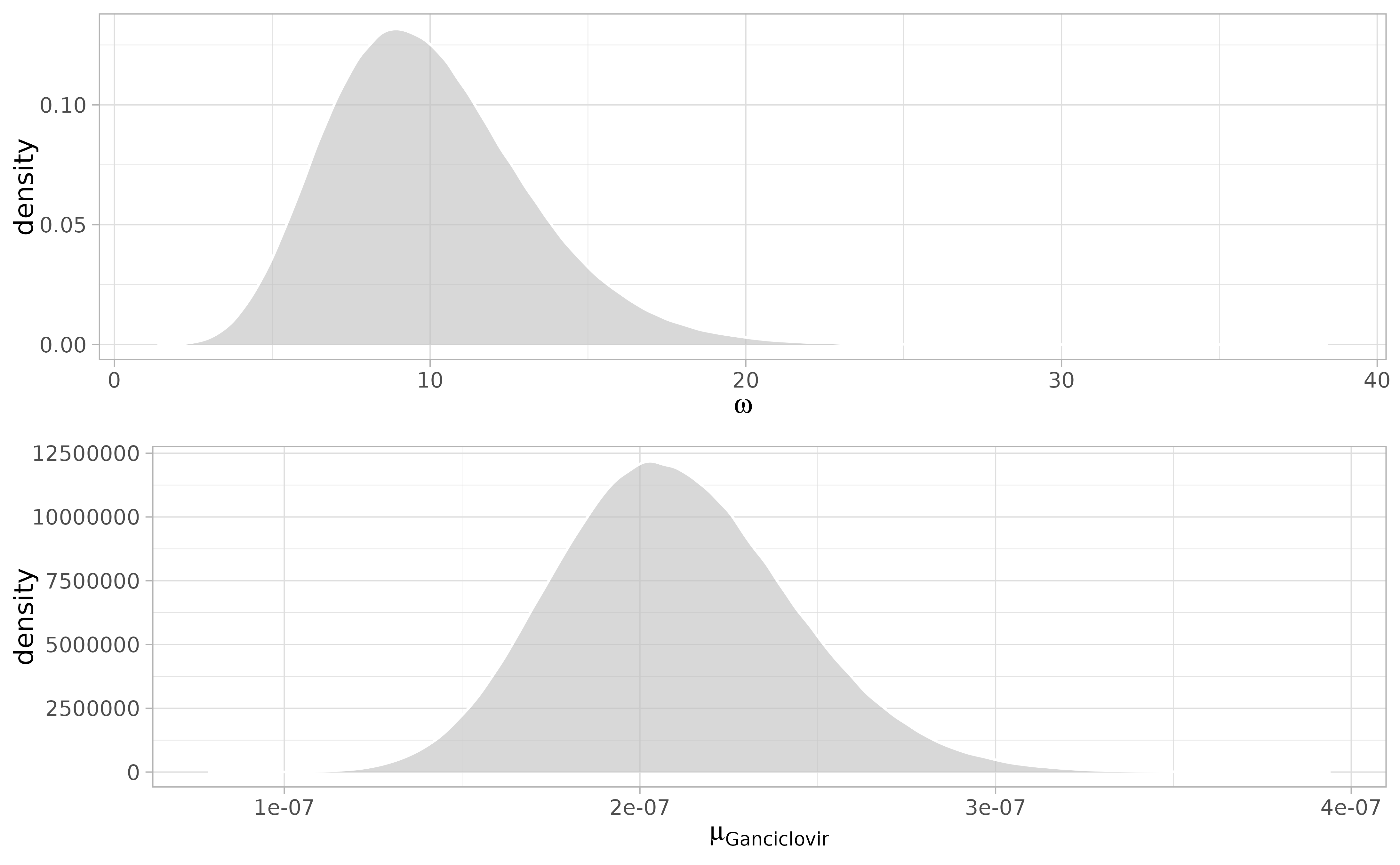

Tumour cell count bounds

The minimum and maximum number of cells in the relapse lineage at primary sampling and at relapse constrain the support of the timing inference. The defaults ( $10^6$ and $10^{13}$ ) can be adjusted if clinical or biological information suggests otherwise. Users can also specify whether to apply a likelihood regularisation term assuming exponential growth before the first and/or second sample, via the exponential_growth parameter, which takes value 1 (enabled) or 0 (disabled) for each sample independently. For UPN06:

UPN06$Input$Parameters %>% 
  filter(Name %in% c("exponential_growth", "N_min", "N_max"))
#>                 Name Value          Index
#> 1 exponential_growth 0e+00 Pre-Transplant
#> 2 exponential_growth 1e+00        Relapse
#> 3              N_min 1e+06 Pre-Transplant
#> 4              N_max 1e+13 Pre-Transplant
#> 5              N_min 1e+08        Relapse
#> 6              N_max 1e+11        Relapse

Optional parameters

Two additional parameters allow finer control over the model behaviour. k_step controls how sharply therapy-associated mutagenesis turns on and off: rather than an instantaneous switch at the start/end of treatment, the rate transitions smoothly, which also keeps the model differentiable for the sampler. The phi_* parameters relax the base Poisson assumption (mean equals variance) to a Negative-Binomial one, adding an overdispersion term for each mutation group so that counts noisier than a pure Poisson process would allow don’t bias the timing estimates. For UPN06:

UPN06$Input$Parameters %>% 
  filter(Name %in% c("k_step", "phi_clock", "phi_th_step", "phi_cna_alpha", "phi_cna_beta"))
#>            Name   Value       Index
#> 1        k_step 2.5e+03        <NA>
#> 2     phi_clock 1.0e-03        <NA>
#> 3   phi_th_step 1.0e-03 Ganciclovir
#> 4 phi_cna_alpha 1.0e-03    47911693
#> 5  phi_cna_beta 1.0e-03    47911693