Running the inference
See the Overview vignette for the core idea and a glossary of the terms used below.
Once all inputs are in place and the TOSCA object has been correctly
initialised, the inference is launched with a single call to
fit(). The function takes the TOSCA object as input and
populates its inference results slot. For resistances mediated by a CNA
event, as is the case for UPN06, model_name should be set
to "CNA"; for resistance mediated by a driver mutation (see
vignette 2), use "Driver" instead. The
dormancy argument should be set to TRUE when
the patient has received a chemotherapeutic agent known to induce tumour
cell dormancy, such as cytarabine. Additional arguments allow
fine-grained control over the MCMC sampler (number of chains, iterations
per chain, warmup length, and so on); see ?TOSCA::fit for
full details.
Should you trust the result?
Always check the convergence report before trusting a
fit() result — an inference that hasn’t converged shouldn’t
be interpreted, regardless of how plausible the numbers look. That said,
TOSCA’s classification of pre-existing versus de novo resistance has
held up well under scrutiny: validated on simulated tumour evolution
with a known ground truth, across both copy-number- and
mutation-mediated resistance, and under deliberate violations of the
model’s own assumptions (e.g. non-constant growth rates), it correctly
classified pre-existing versus de novo resistance in roughly 94–98% of
simulated cases. In the real haematological cases studied in the
reference paper, several TOSCA-inferred timings were independently
corroborated by mutational-signature evidence never shown to the model
during fitting.
UPN06 <- TOSCA::fit(
  UPN06,
  model_name = "CNA",
  dormancy   = TRUE
)
Upon completion, fit() prints a summary report
containing:
- Convergence diagnostics: whether all , the number of divergent transitions, and whether the E-BFMI fell below 0.3 in any chain.
- Preliminary posterior predictive check: whether the observed mutation count for each group falls between the mode and the 90th percentile of the posterior predictive distribution.
- Parameter summary: posterior estimates for each inferred parameter, including the posterior predictives.
A summary of the inference results can be retrieved at any time with:
TOSCA::get_fit_summary(UPN06)
#> # A tibble: 12 × 7
#>    variable        median      mean              rhat ess_bulk q5          q95
#>    <chr>           <chr>       <chr>            <dbl>    <dbl> <chr>       <chr>
#>  1 t_eca           2012-4-2    2012-3-30        1.00    11731. 2012-1-1    2012…
#>  2 t_mrca_primary  2012-4-2    2012-3-30        1.00    11731. 2012-1-1    2012…
#>  3 t_dormancy_end  2014-2-19   2014-2-21        1.00    11538. 2013-12-13  2014…
#>  4 omega           10.8337     10.88481265825   1.00    11159. 9.4005805   12.5…
#>  5 mu_Ganciclovir  2.25783e-07 2.2679160095e-07 1.00    12368. 1.9433595e… 2.62…
#>  6 t_mrca          2014-8-10   2014-8-9         1.00    20467. 2014-7-6    2014…
#>  7 t_cna[1]        2014-7-27   2014-7-28        1.00    21663. 2014-6-27   2014…
#>  8 m_clock_primary 1           1.100025         1.00    31916. 0           4
#>  9 m_clock         844         845.2797         1.000   43382. 756         939
#> 10 m_gcv           1341        1343.471575      1.00    42739. 1218        1475
#> 11 alpha           18          18.102825        1.00    39197. 11          26
#> 12 beta            1           1.732275         1.00    30784. 0           5
The fitted object also exposes the raw posterior draws, model specification, and diagnostic summary directly:
UPN06$Fit$posteriors
#> $stan_posterior
#> # A draws_df: 10000 iterations, 4 chains, and 35 variables
#>    lp__ t_eca t_mrca_primary t_dormancy_end t_mrca_tr t_cna_tr[1] omega
#> 1  -680    58             58             60        58          58   9.1
#> 2  -682    58             58             60        58          58  10.8
#> 3  -677    58             58             60        58          58  10.0
#> 4  -676    58             58             60        58          58  10.3
#> 5  -677    58             58             60        58          58  10.2
#> 6  -675    58             58             60        59          59  10.5
#> 7  -676    58             58             60        59          59  11.7
#> 8  -673    58             58             60        58          58  10.6
#> 9  -676    58             58             60        58          58  12.0
#> 10 -673    58             58             60        58          58  11.0
#>    mu_th_step[1]
#> 1        2.5e-07
#> 2        2.4e-07
#> 3        2.2e-07
#> 4        2.2e-07
#> 5        2.2e-07
#> 6        2.3e-07
#> 7        2.0e-07
#> 8        2.4e-07
#> 9        2.0e-07
#> 10       2.2e-07
#> # ... with 39990 more draws, and 27 more variables
#> # ... hidden reserved variables {'.chain', '.iteration', '.draw'}
#>
#> $timing_posteriors
#> # A tibble: 40,000 × 5
#>    t_eca      t_mrca_primary t_dormancy_end t_mrca    `t_cna[1]`
#>    <chr>      <chr>          <chr>          <chr>     <chr>
#>  1 2012-1-5   2012-1-6       2014-4-2       2014-7-2  2014-6-21
#>  2 2011-12-25 2011-12-26     2014-5-18      2014-8-14 2014-7-26
#>  3 2011-12-28 2011-12-28     2014-5-17      2014-8-10 2014-7-27
#>  4 2012-1-5   2012-1-5       2014-5-13      2014-8-15 2014-8-9
#>  5 2012-1-1   2012-1-1       2014-5-14      2014-8-10 2014-8-5
#>  6 2012-4-27  2012-4-27      2014-2-22      2014-8-28 2014-8-8
#>  7 2012-6-27  2012-6-27      2013-12-22     2014-8-24 2014-8-16
#>  8 2012-2-27  2012-2-27      2014-3-29      2014-8-20 2014-8-3
#>  9 2012-2-12  2012-2-12      2014-5-6       2014-9-3  2014-8-26
#> 10 2012-2-18  2012-2-18      2014-3-28      2014-7-27 2014-7-9
#> # ℹ 39,990 more rows
#>
#> $posterior_predictive_checks
#> # A tibble: 40,000 × 5
#>    m_clock_primary m_clock m_gcv alpha  beta
#>              <dbl>   <dbl> <dbl> <dbl> <dbl>
#>  1               1     739  1292    14     3
#>  2               1     997  1316    15     2
#>  3               0     855  1179    26     1
#>  4               0     827  1269    11     0
#>  5               1     801  1277    20     1
#>  6               0     785  1324    16     3
#>  7               0     908  1223    12     2
#>  8               2     911  1372    18     4
#>  9               1     953  1296    22     0
#> 10               0     774  1394    19     3
#> # ℹ 39,990 more rows
#>
#> $rates_posteriors
#> # A tibble: 40,000 × 2
#>    omega mu_Ganciclovir
#>    <dbl>          <dbl>
#>  1  9.10    0.000000248
#>  2 10.8     0.000000237
#>  3  9.96    0.000000221
#>  4 10.3     0.000000219
#>  5 10.2     0.000000220
#>  6 10.5     0.000000229
#>  7 11.7     0.000000195
#>  8 10.6     0.000000239
#>  9 12.0     0.000000201
#> 10 11.0     0.000000217
#> # ℹ 39,990 more rows
#>
#> $stan_fit
#>               variable    mean  median   sd  mad      q5     q95 rhat ess_bulk
#>  lp__                  -674.94 -674.60 1.86 1.70 -678.48 -672.57 1.00    12700
#>  t_eca                   58.25   58.25 0.15 0.17   58.00   58.48 1.00    11731
#>  t_mrca_primary          58.25   58.25 0.15 0.17   58.00   58.48 1.00    11730
#>  t_dormancy_end          60.14   60.13 0.13 0.17   59.94   60.36 1.00    11538
#>  t_mrca_tr               58.54   58.55 0.15 0.17   58.30   58.77 1.00    11653
#>  t_cna_tr[1]             58.51   58.52 0.15 0.17   58.27   58.74 1.00    11733
#>  omega                   10.88   10.83 0.96 1.03    9.40   12.50 1.00    11159
#>  mu_th_step[1]            0.00    0.00 0.00 0.00    0.00    0.00 1.00    12368
#>  lambda_th_step[1]        0.10    0.10 0.00 0.00    0.09    0.10 1.00    12376
#>  lambda_alpha_clock[1]    6.50    6.57 0.65 0.60    5.30    7.41 1.00    24882
#>  ess_tail
#>     17051
#>     22048
#>     21904
#>     17342
#>     20559
#>     21589
#>     19541
#>     20515
#>     11976
#>     28020
#>
#>  # showing 10 of 35 rows (change via 'max_rows' argument or 'cmdstanr_max_rows' option)
UPN06$Fit$model_info
#> $model_name
#> [1] "CNA"
#>
#> $dormancy
#> [1] TRUE
UPN06$Fit$diagnostic_summary
#> $num_divergent
#> [1] 0 0 0 0
#>
#> $num_max_treedepth
#> [1] 2 0 3 0
#>
#> $ebfmi
#> [1] 1.0436962 1.0174633 1.0209456 0.9769555
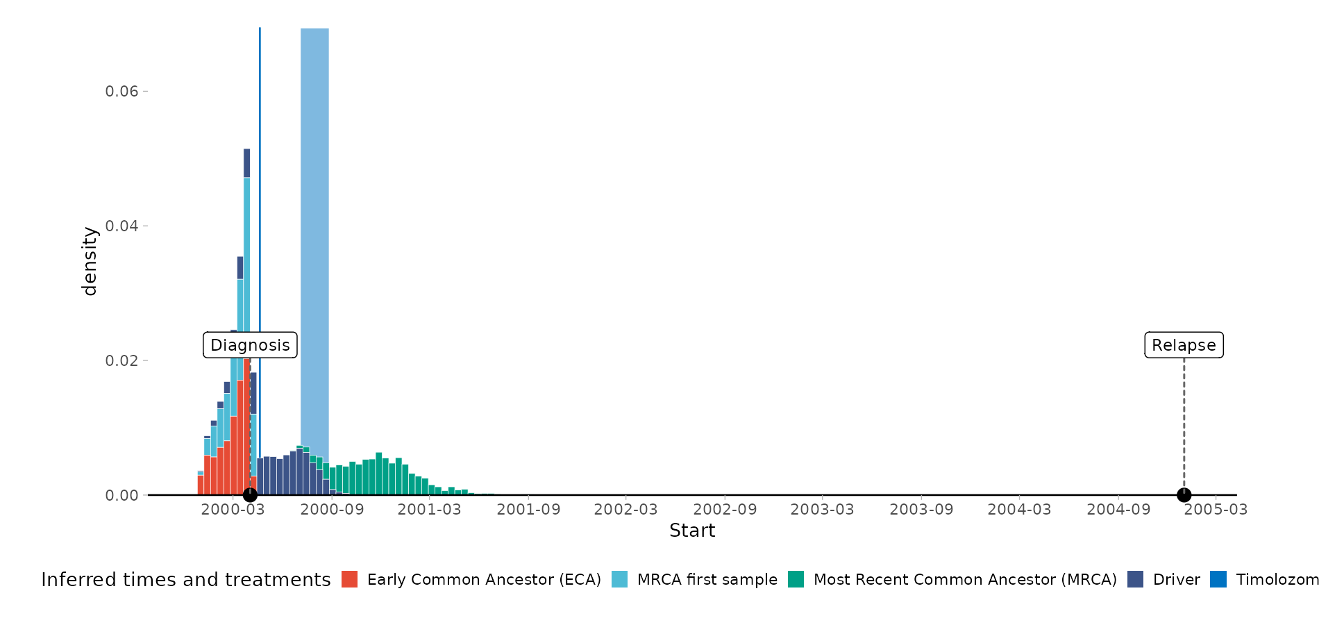
Watching it actually run
The examples above use pre-computed results, since a real fit on
WGS-scale data takes a while. To see the whole pipeline —
init() then fit() then a plot — actually
execute, here it is live on exampleData_Driver, the toy
driver-model dataset from the previous vignette. It’s small enough to
sample in a few seconds even with a real, not pre-computed, fit:
data("exampleData_Driver")

toy <- init(
  mutations   = exampleData_Driver$Input$Mutations,
  samples     = exampleData_Driver$Input$Samples,
  therapies   = exampleData_Driver$Input$Therapies,
  parameters  = exampleData_Driver$Input$Parameters,
  sample_name = "toy-driver"
)

toy <- fit(
  toy,
  model_name   = "Driver",
  n_chains     = 2,
  n_iterations = 800,
  warm_up      = 500
)
#>
#> --- Start Sampling ---
#>
#> --- End Sampling ---
#>
#> --- Sampling Diagnostics ---
#> Convergence (Rhat < 1.01): ✅ Yes (max Rhat = 1.008)
#> Divergent transitions: 0 / 1600 (0.00%)
#> EBFMI < 0.3 in 0 / 2 chains
#>
#> --- Posterior Predictive Checks ---
#>           name pass
#> 1 sbs1_primary TRUE
#> 2 sbs1_relapse TRUE
#> 3        sbs11 TRUE
#>
#> --- Inference summary ---
#>          variable         median                mean     rhat  ess_bulk
#> 1           t_eca       2000-3-8           2000-2-28 1.002330  778.6061
#> 2  t_mrca_primary      2000-3-17            2000-3-9 1.006269  691.2371
#> 3       mu_driver 4.62863585e-08 4.8260910021875e-08 1.001284  796.0054
#> 4           omega      4.9445061      4.974460772625 1.003706  864.0282
#> 5          t_mrca     2000-11-25          2000-11-30 1.000567  708.0581
#> 6        t_driver      2000-5-27           2000-5-24 1.002252  535.9155
#> 7 m_clock_primary              0               0.745 1.001269 1586.7671
#> 8         m_clock             76             83.1875 1.002083 1210.8278
#> 9        m_driver            155           168.86875 1.000188 1166.0992
#>               q5             q95
#> 1      2000-1-10        2000-4-1
#> 2      2000-1-22        2000-4-2
#> 3 2.95827131e-08 7.303974405e-08
#> 4     4.53292796     5.538601255
#> 5      2000-8-13        2001-4-8
#> 6      2000-2-24       2000-8-13
#> 7              0               3
#> 8             34             161
#> 9             74          313.05
These are deliberately reduced settings, fine for a toy dataset this small and fast to run here, but not representative of what a real analysis should use — the earlier UPN06 example’s defaults (4 chains, 10000 iterations, 5000 warmup) are a more realistic starting point for WGS-scale data. Even so, notice the convergence report above: this small run already converges cleanly. A first look at the result, using the plotting functions from the next vignette:
plot_timing(toy)