Note: This article presents advanced topics on tissue simulation. Refer to this article for an introduction on the subject.
Disclaimer: ProCESS/CLONES internally implements the probability distributions using the C++11 random number distribution classes. The standard does not specify their algorithms, and the class implementations are left free for the compiler. Thus, the simulation output depends on the compiler used to compile CLONES, and because of that, the results reported in this article may differ from those obtained by the reader.
Sometimes it is convenient to plot a time series of a simulation, reporting species or firing counts over time. Since ProCESS is programmable, it is easy to make a for-loop algorithm and collect the simulation data over time.
Default History-Based Data
However, this is not required because at the end of any
run_to_* method, CLONES stores data on the number of
species cells and the number of event firings. These data can be
extracted.
Let us consider the simulation sim as produced in this article.
library(ProCESS)
library(dplyr)
#>
#> Attaching package: 'dplyr'
#> The following objects are masked from 'package:stats':
#>
#>     filter, lag
#> The following objects are masked from 'package:base':
#>
#>     intersect, setdiff, setequal, union

# The firings
sim$get_firing_history() %>% head()
#>    event mutant epistate fired     time
#> 1  death      A        -    15 58.75396
#> 2 growth      A        -   101 58.75396
#> 3 switch      A        -     9 58.75396
#> 4  death      A        +   793 58.75396
#> 5 growth      A        +  1341 58.75396
#> 6 switch      A        +    58 58.75396

# For example, total number of the deaths on `B+` at the end of the
# previous calls of the `run_to_*` methods
sim$get_firing_history() %>%
  filter(event == "death", mutant == "B", epistate == "-")
#>   event mutant epistate fired      time
#> 1 death      B        -     0  58.75396
#> 2 death      B        -     0  85.92293
#> 3 death      B        -     0 100.92305
#> 4 death      B        -   465 143.82685
#> 5 death      B        -   733 150.82736

# The counts
sim$get_count_history() %>% head()
#>   mutant epistate count     time
#> 1      A        -   135 58.75396
#> 2      A        +   500 58.75396
#> 3      B        -     0 58.75396
#> 4      B        +     0 58.75396
#> 5      C        -     0 58.75396
#> 6      C        +     0 58.75396
The time-series can be plot using plot_timeseries()
# Time-series plot
plot_timeseries(sim)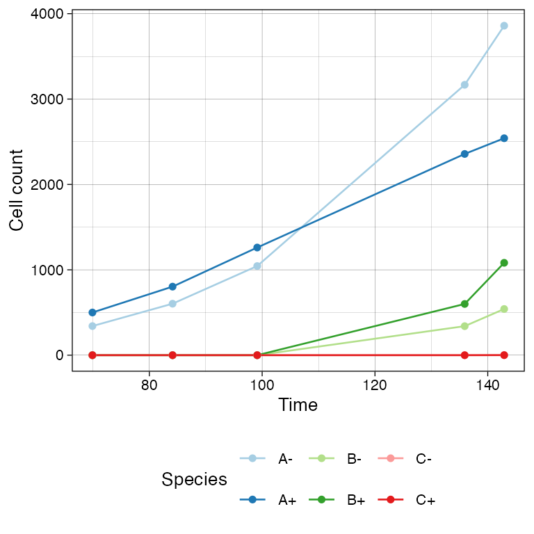
Custom Time-Series
If the default time-series is not enough coarse-grained, one can set
TissueSimulationhistory_delta](../reference/TissueSimulation-cash-history_delta.html)</code>
to increase the sampling rate of
the state (by default,
<code>[TissueSimulationhistory_delta
is set to
0).
We show this by re-simulating a tumour with two sub-mutants.
# Example time-series on a new simulation, with coarse-grained time-series
sim <- TissueSimulation("Finer Time Series")

sim$history_delta <- 1
sim$death_activation_level <- 100

# A
sim$add_mutant(name = "A",
               epigenetic_rates = c("+-" = 0.01, "-+" = 0.01),
               growth_rates = c("+" = 0.2, "-" = 0.08),
               death_rates = c("+" = 0.1, "-" = 0.01))

sim$place_cell("A+", 500, 500)
sim$run_up_to_size("A+", 400)
#>  [████████████████████████████████████████] 100% [00m:00s] Saving snapshot

# B (linear inside A)
sim$add_mutant(name = "B",
               epigenetic_rates = c("+-" = 0.05, "-+" = 0.05),
               growth_rates = c("+" = 0.3, "-" = 0.3),
               death_rates = c("+" = 0.05, "-" = 0.1))

sim$mutate_progeny(sim$choose_cell_in("A"), "B")

sim$run_up_to_size("B-", 300)
#>  [████████████████████████████████████████] 100% [00m:00s] Saving snapshot

# C (linear inside B)
sim$add_mutant(name = "C",
               epigenetic_rates = c("+-" = 0.1, "-+" = 0.1),
               growth_rates = c("+" = 0.2, "-" = 0.4),
               death_rates = c("+" = 0.1, "-" = 0.01))

sim$mutate_progeny(sim$choose_cell_in("B"), "C")

# D (linear inside A, so branching with C) - same parameters of C
sim$add_mutant(name = "D",
               epigenetic_rates = c("+-" = 0.1, "-+" = 0.1),
               growth_rates = c("+" = 0.2, "-" = 0.4),
               death_rates = c("+" = 0.1, "-" = 0.01))

sim$mutate_progeny(sim$choose_cell_in("A"), "D")

sim$run_up_to_size("D+", 1000)
#>  [████████████████████████████████--------] 78% [00m:00s] Cells: 29274 [████████████████████████████████████████] 100% [00m:00s] Saving snapshot
The time-series can be plot using plot_timeseries().
# Time-series plot
plot_timeseries(sim)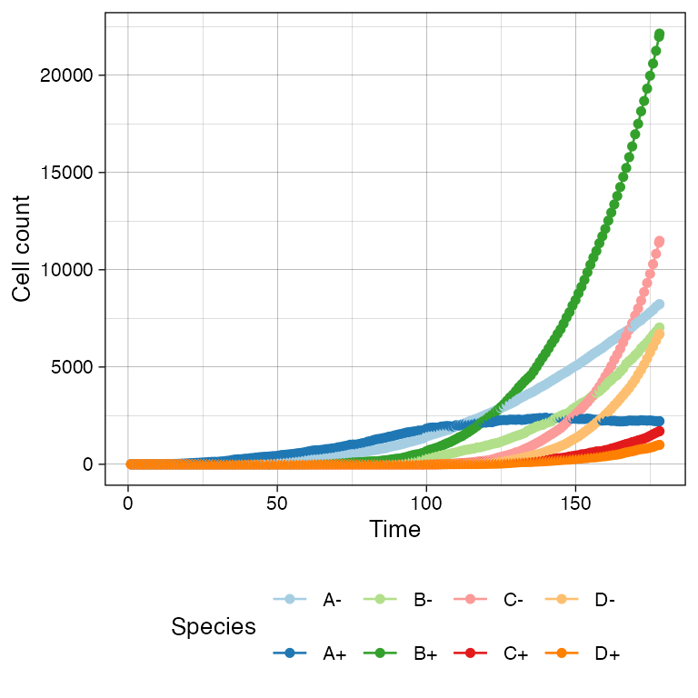
# Logscale helps seeing the different effective growth rates
plot_timeseries(sim) + ggplot2::scale_y_log10()
#> Warning in ggplot2::scale_y_log10(): log-10 transformation introduced infinite values.
#> log-10 transformation introduced infinite values.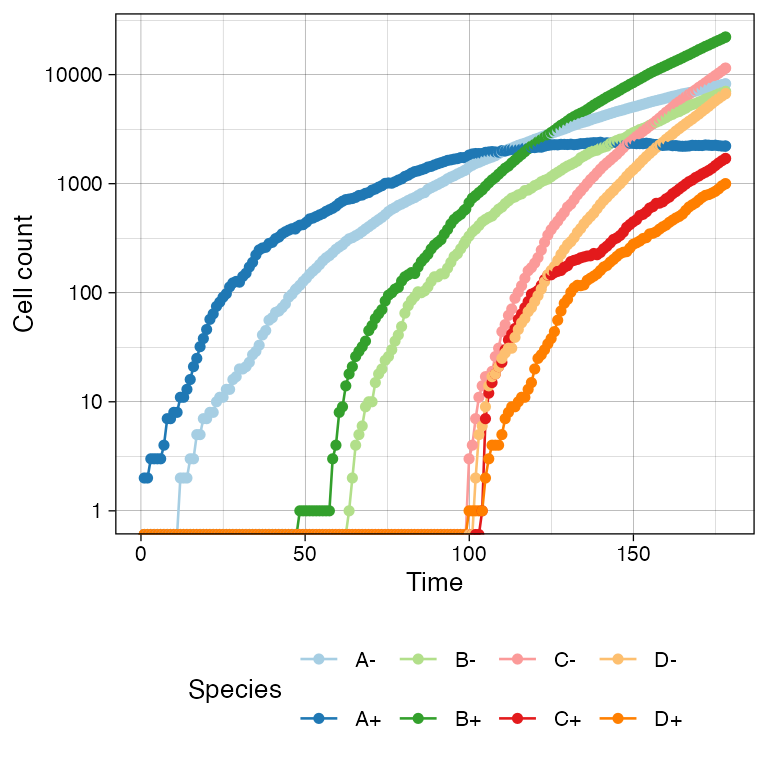
Muller Plot
We can also get a Muller plot of the evolution using ggmuller.
# default Muller plot
plot_muller(sim)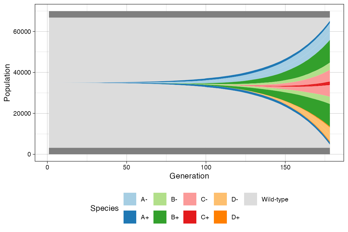
In this case every population is annotated as a descendant of the ancestor mutant. Note however that reversible epi-states do not fit a traditional Muller plot because they violate the no-back mutation model.
In this case, ProCESS will show first the epi-state that was randomly injected in the simulation, and the second will result by linear. This is not a completely correct perspective of the simulation time-series; still, it help understand trends.
# Custom Mullers
clock <- sim$get_clock()

plot_muller(sim) + ggplot2::xlim(clock * 3/4, clock)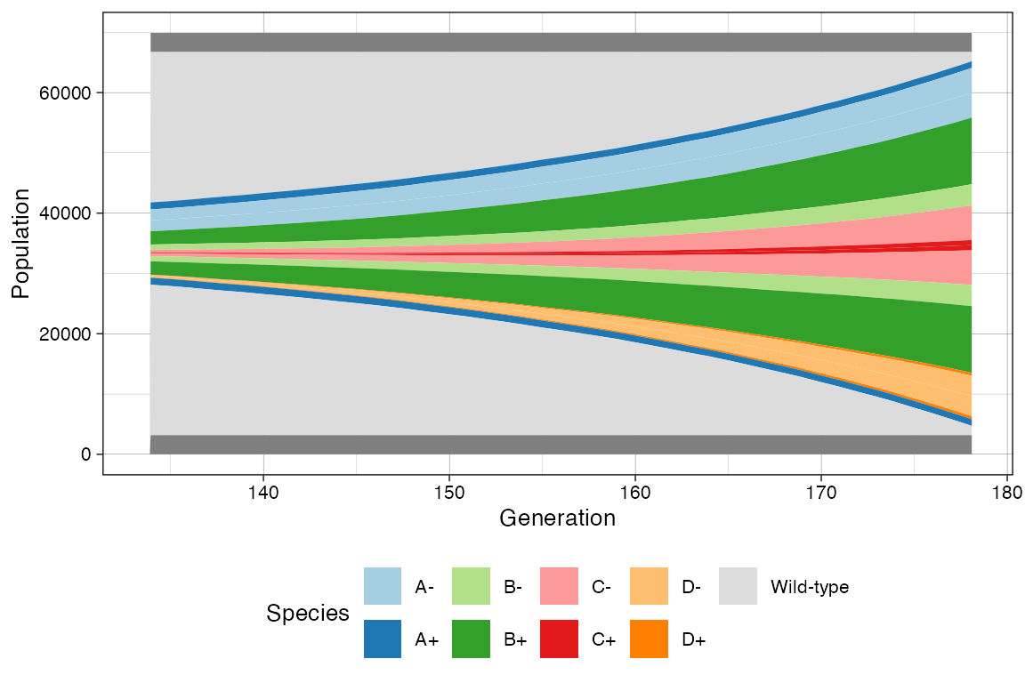
plot_muller(sim) +
  ggplot2::xlim(clock * 3/4, clock) +
  ggplot2::scale_y_log10()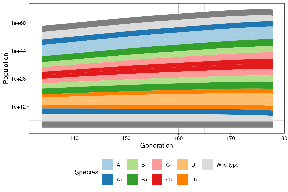
Time-Varying Evolutionary Rates
The rates of any species may change over time. For instance, this happens when a population is subject to a targeted treatment.
For instance, going back to the example simulation, we can increase
the death rates of C+, C-, B+,
and B-.
# Current rates
sim
#>
#> ======= ==== ==== ==== ====== =========
#> species λ δ ε counts %
#> ======= ==== ==== ==== ====== =========
#> A- 0.08 0.01 0.01 3510 10.223400
#> A+ 0.20 0.10 0.01 958 2.790318
#> B- 0.30 0.10 0.05 2712 7.899106
#> B+ 0.30 0.05 0.05 9800 28.543966
#> C- 0.40 0.01 0.10 7303 21.271080
#> C+ 0.20 0.10 0.10 770 2.242740
#> D- 0.40 0.01 0.10 8280 24.116739
#> D+ 0.20 0.10 0.10 1000 2.912650
#> ======= ==== ==== ==== ====== =========
#>
#> Species [A-]: 2158 (deaths), 5517 (duplications) and 601 (switches)
#> Species [A+]: 14341 (deaths), 15451 (duplications) and 752 (switches)
#> Species [B-]: 13994 (deaths), 13652 (duplications) and 1935 (switches)
#> Species [B+]: 22240 (deaths), 35094 (duplications) and 4989 (switches)
#> Species [C-]: 1699 (deaths), 10505 (duplications) and 2059 (switches)
#> Species [C+]: 2434 (deaths), 1700 (duplications) and 556 (switches)
#> Species [D-]: 2065 (deaths), 12027 (duplications) and 2361 (switches)
#> Species [D+]: 2706 (deaths), 2023 (duplications) and 679 (switches)
# Raise the death rate levels
sim$update_rates("B+", c(death = 0.5))
sim$update_rates("B-", c(death = 0.5))
sim$update_rates("C+", c(death = 0.5))
sim$update_rates("C-", c(death = 0.5))
# Now D will become larger
sim$run_up_to_size("D+", 6000)
#> [████████████----------------------------] 28% [00m:00s] Cells: 25158 [█████████████████████████---------------] 61% [00m:00s] Cells: 50983 [█████████████████████████████████████---] 91% [00m:01s] Cells: 80454 [████████████████████████████████████████] 100% [00m:02s] Saving snapshot
# Current state
sim
#>
#> ======= ==== ==== ==== ====== =========
#> species λ δ ε counts %
#> ======= ==== ==== ==== ====== =========
#> A- 0.08 0.01 0.01 6529 7.341069
#> A+ 0.20 0.10 0.01 1043 1.172727
#> B- 0.30 0.50 0.05 0 0.000000
#> B+ 0.30 0.50 0.05 0 0.000000
#> C- 0.40 0.50 0.10 0 0.000000
#> C+ 0.20 0.50 0.10 0 0.000000
#> D- 0.40 0.01 0.10 75366 84.739931
#> D+ 0.20 0.10 0.10 6000 6.746273
#> ======= ==== ==== ==== ====== =========
#>
#> Species [A-]: 7311 (deaths), 14089 (duplications) and 1520 (switches)
#> Species [A+]: 25141 (deaths), 25936 (duplications) and 1271 (switches)
#> Species [B-]: 25313 (deaths), 21142 (duplications) and 3046 (switches)
#> Species [B+]: 46803 (deaths), 50974 (duplications) and 7217 (switches)
#> Species [C-]: 44011 (deaths), 50731 (duplications) and 10056 (switches)
#> Species [C+]: 16770 (deaths), 10049 (duplications) and 3336 (switches)
#> Species [D-]: 36903 (deaths), 131370 (duplications) and 26238 (switches)
#> Species [D+]: 34428 (deaths), 21326 (duplications) and 7137 (switches)
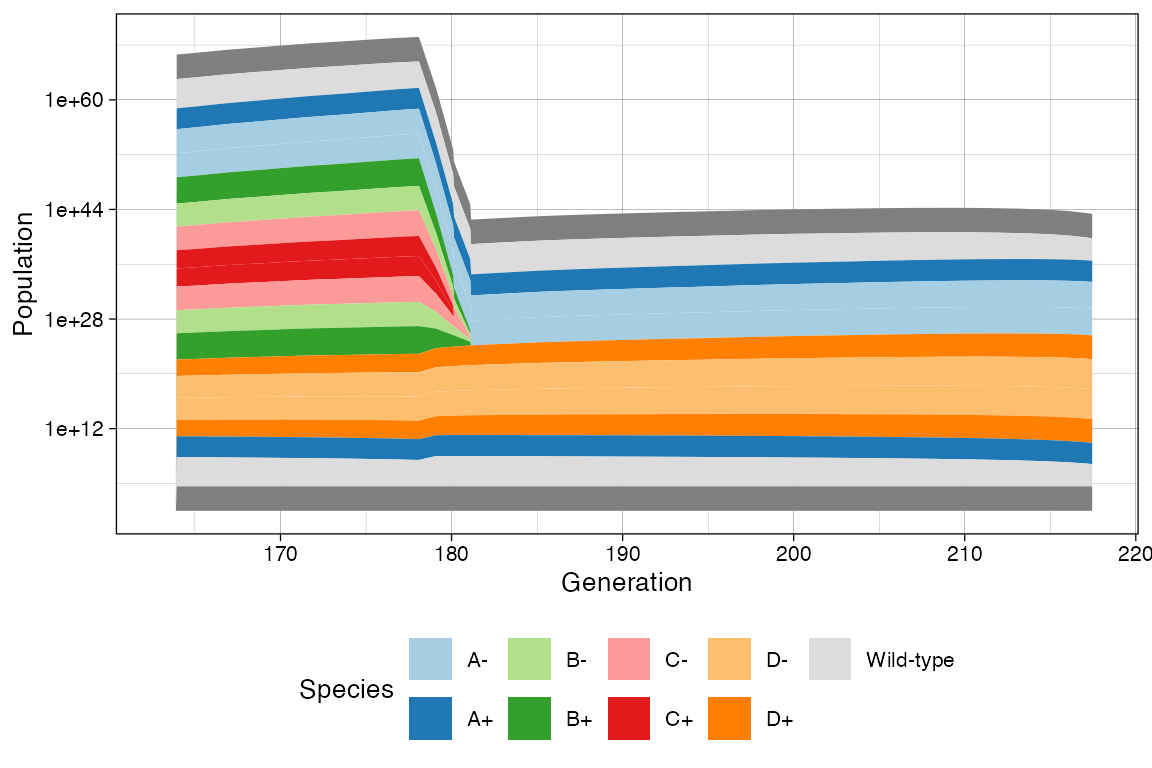
# This now show the change in rates
clock <- sim$get_clock()
plot_muller(sim) + ggplot2::xlim(clock * 3/4, clock)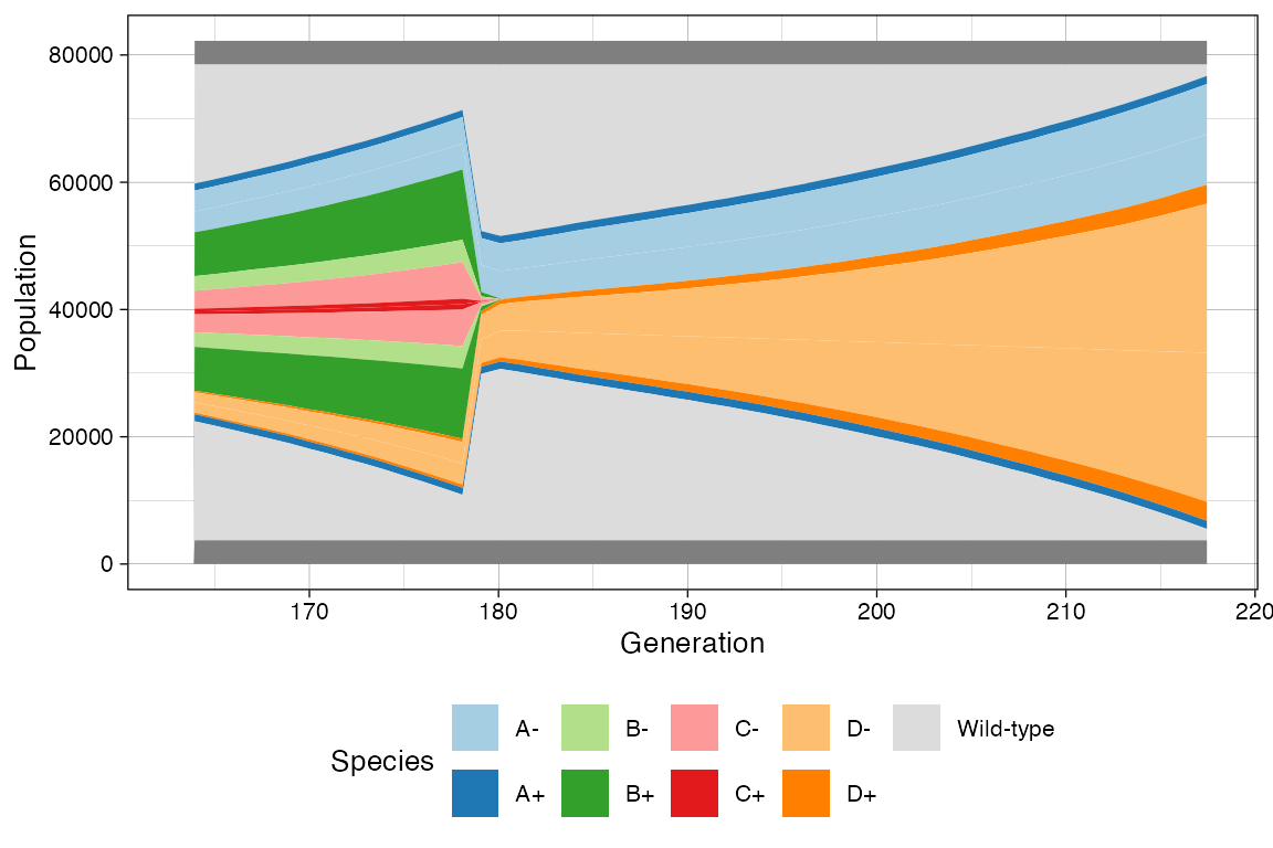
plot_muller(sim) +
  ggplot2::xlim(clock * 3/4, clock) +
  ggplot2::scale_y_log10()