2. Inference of mutation copy number and multiplicity • INCOMMON

library(INCOMMON)
#> Warning: replacing previous import 'cli::num_ansi_colors' by
#> 'crayon::num_ansi_colors' when loading 'INCOMMON'
library(dplyr)
#> 
#> Attaching package: 'dplyr'
#> The following objects are masked from 'package:stats':
#> 
#>     filter, lag
#> The following objects are masked from 'package:base':
#> 
#>     intersect, setdiff, setequal, union
library(DT)
library(cli)
library(crayon)
#> 
#> Attaching package: 'crayon'
#> The following object is masked from 'package:cli':
#> 
#>     num_ansi_colors

In this vignette, we use INCOMMON to infer the copy number and multiplicity of mutations from a single sample of the MSK-MetTropsim dataset provided within the package.

2.1 Input preparation

The minimal input for INCOMMON analyses consists of two pieces.

2.1.1 Genomic data

First we need a table of genomic_data (mutations) with required columns chr, from, to, ref, alt, DP, NV, VAF, and gene.

The following example is taken from the internal dataset obtained from the MSK-MetTropism cohort:

2.1.2 Clinical data

Second, we need a table of clinical data with at least the columns sample (sample names matching the ones in genomic_data), purity (purity of each sample) and tumor_type (annotated tumour type of the sample), required for using tumour-specific priors. The following example is taken from the internal dataset obtained from the MSK-MetTropism cohort:

2.1.3 Initialisation of the input

The first thing to do is to initialise the input so that we will have it in INCOMMON format, through function init. This function takes as input the tables of genomic_data and clinical_data, plus optionally, a list of gene roles.

INCOMMON provides a default list cancer_gene_census obtained from the COSMIC Cancer Gene Census v.98. The required format is as following:

We now can create the input INCOMMON object through the function init:

x = init(genomic_data = MSK_genomic_data, 
         clinical_data = MSK_clinical_data, 
         gene_roles = cancer_gene_census)
#> ── INCOMMON - Inference of copy number and mutation multiplicity in oncology ───
#> 
#> ── Genomic data ──
#> 
#> ✔ Found 25659 samples, with 224939 mutations in 491 genes
#> ! No read counts found for 1393 mutations in 1393 samples
#> ! Gene name not provided for 1393 mutations
#> ! 201 genes could not be assigned a role (TSG or oncogene)
#> 
#> ── Clinical data ──
#> 
#> ℹ Provided clinical features:
#> ✔ sample (required for classification)
#> ✔ purity (required for classification)
#> ✔ tumor_type
#> ✔ OS_MONTHS
#> ✔ OS_STATUS
#> ✔ SAMPLE_TYPE
#> ✔ MET_COUNT
#> ✔ METASTATIC_SITE
#> ✔ MET_SITE_COUNT
#> ✔ PRIMARY_SITE
#> ✔ SUBTYPE_ABBREVIATION
#> ✔ GENE_PANEL
#> ✔ SEX
#> ✔ TMB_NONSYNONYMOUS
#> ✔ FGA
#> ✔ AGE_AT_SEQUENCING
#> ✔ RACE
#> ✔ Found 25257 matching samples
#> ✖ Found 513 unmatched samples

print(x)
#> ── [ INCOMMON ]  175054 PASS mutations across 24018 samples, with 290 mutant gen
#> ℹ Average sample purity: 0.4
#> ℹ Average sequencing depth: 649
#> # A tibble: 175,054 × 27
#>    sample    tumor_type purity chr     from     to ref   alt      DP    NV   VAF
#>    <chr>     <chr>       <dbl> <chr>  <dbl>  <dbl> <chr> <chr> <int> <int> <dbl>
#>  1 P-0028912 CHOL          0.3 chr17 7.58e6 7.58e6 G     A       837   133 0.159
#>  2 P-0028912 CHOL          0.3 chrX  5.32e7 5.32e7 G     A       832    85 0.102
#>  3 P-0003698 BLCA          0.2 chr17 7.58e6 7.58e6 C     A       437   109 0.249
#>  4 P-0003698 BLCA          0.2 chr5  1.49e8 1.49e8 C     T       360    36 0.1  
#>  5 P-0003698 BLCA          0.2 chr13 3.29e7 3.29e7 G     C      1027   162 0.158
#>  6 P-0003698 BLCA          0.2 chr13 3.29e7 3.29e7 G     C      1021   182 0.178
#>  7 P-0003698 BLCA          0.2 chr19 1.11e7 1.11e7 G     T       573    98 0.171
#>  8 P-0003698 BLCA          0.2 chr22 4.15e7 4.15e7 G     A       416    45 0.108
#>  9 P-0003698 BLCA          0.2 chrX  4.49e7 4.49e7 C     T       730   194 0.266
#> 10 P-0003823 BLCA          0.6 chr5  1.30e6 1.30e6 G     A       218   138 0.633
#> # ℹ 175,044 more rows
#> # ℹ 16 more variables: gene <chr>, gene_role <chr>, OS_MONTHS <dbl>,
#> #   OS_STATUS <dbl>, SAMPLE_TYPE <chr>, MET_COUNT <dbl>, METASTATIC_SITE <chr>,
#> #   MET_SITE_COUNT <dbl>, PRIMARY_SITE <chr>, SUBTYPE_ABBREVIATION <chr>,
#> #   GENE_PANEL <chr>, SEX <chr>, TMB_NONSYNONYMOUS <dbl>, FGA <dbl>,
#> #   AGE_AT_SEQUENCING <dbl>, RACE <chr>

The MSK-MET dataset comprises 25257 samples with matched clinical data. The average sequencing depth is 649 and the average sample purity is 0.4. The 175054 mutations flagged as PASS are the ones that satisfy the requirements for INCOMMON classification: available and non-negative sample purity; integer sequencing depth and number of reads with the variant, character gene names etc.

2.2 Inference of copy number and mutation multiplicity

In principle, INCOMMON can infer any configuration of total copy number k and mutation multiplicity m, given that both k and m are integer numbers and $m\leq k$ . Since there is an infinite number of such possible configurations, a maximum value k_max of k, expected to be found in the dataset, must be set up prior to the classification task. By default, INCOMMON uses $k_{max}=8$ .

2.2.1 Rate of read counts per chromosome copy

INCOMMON is a Bayesian model that infers mutation copy number and multiplicity from read counts. An essential parameter of the model is the rate of read counts per chromosome copy $\eta$ . To guide the inference of this parameter, we use a Gamma prior distribution. The only a priori information that we have access to is on the $(k,m)$ configurations of mutant genes. We use this to compute a prior distribution over $\eta$ from the dataset itself, using the functioncompute_eta_prior

data('priors_pcawg_hmf')

priors_eta = compute_eta_prior(x = x, priors_k_m = priors_pcawg_hmf)
print(priors_eta)
#> # A tibble: 12 × 6
#>    tumor_type mean_eta var_eta     N alpha_eta beta_eta
#>    <chr>         <dbl>   <dbl> <int>     <dbl>    <dbl>
#>  1 BRCA           320.  31113.  2271      3.28  0.0103 
#>  2 ESCA           357.  28769.   285      4.44  0.0124 
#>  3 GIST           340.  61998.   299      1.87  0.00549
#>  4 HCC            304.  16885.   171      5.48  0.0180 
#>  5 LUAD           353.  34458.  3406      3.61  0.0102 
#>  6 MEL            304.  28999.  1042      3.19  0.0105 
#>  7 OV             316.  19945.   936      5.01  0.0159 
#>  8 PAAD           334.  15101.  1698      7.38  0.0221 
#>  9 PRAD           283.  21340.   223      3.75  0.0133 
#> 10 SCLC           372.  45882.   255      3.01  0.00811
#> 11 STAD           298.  17672.    85      5.04  0.0169 
#> 12 PANCA          332.  29352. 10732      3.75  0.0113

For each tumour type in the dataset, we estimated the empirical mean and variance of $\eta$ , which can be straightforwardly transformed into the shape parameters $\alpha_\eta$ and $\beta_eta$ of a Gamma distribution.

We can visualise the prior distribution for each tumour type using the function plot_eta_prior:

plot_eta_prior(x = x, priors_eta = priors_eta)

The plot shows, for each tumour type and at the pan-cancer level (PANCA), the distribution of total read counts, potentially confused by diverse copy-number configurations and sample purities, and the underlying prior distribution of the rate of read counts per chromosome copy.

2.2.2 Inference in sample ‘P-0002081’

We now focus on a specific sample:

sample = 'P-0002081'

x = subset_sample(x = x, sample_list = c(sample))

print(x)
#> ── [ INCOMMON ]  175054 PASS mutations across 24018 samples, with 290 mutant gen
#> ℹ Average sample purity: 0.4
#> ℹ Average sequencing depth: 649
#> # A tibble: 4 × 27
#>   sample    tumor_type purity chr      from     to ref   alt      DP    NV   VAF
#>   <chr>     <chr>       <dbl> <chr>   <dbl>  <dbl> <chr> <chr> <int> <int> <dbl>
#> 1 P-0002081 LUAD          0.6 chr12  2.54e7 2.54e7 C     A       743   378 0.509
#> 2 P-0002081 LUAD          0.6 chr17  7.58e6 7.58e6 G     A       246   116 0.472
#> 3 P-0002081 LUAD          0.6 chr19  1.22e6 1.22e6 C     A       260   122 0.469
#> 4 P-0002081 LUAD          0.6 chr19  1.11e7 1.11e7 -     C       271   133 0.491
#> # ℹ 16 more variables: gene <chr>, gene_role <chr>, OS_MONTHS <dbl>,
#> #   OS_STATUS <dbl>, SAMPLE_TYPE <chr>, MET_COUNT <dbl>, METASTATIC_SITE <chr>,
#> #   MET_SITE_COUNT <dbl>, PRIMARY_SITE <chr>, SUBTYPE_ABBREVIATION <chr>,
#> #   GENE_PANEL <chr>, SEX <chr>, TMB_NONSYNONYMOUS <dbl>, FGA <dbl>,
#> #   AGE_AT_SEQUENCING <dbl>, RACE <chr>

The input data table contains 4 mutations affecting KRAS, TP53, STK11 and SMARCA4 genes. In this sample, all 4 mutations have all the required information. We can see that this is a sample of a metastatic lung adenocarcinoma (LUAD), sequenced through the MSK-IMPACT targeted panel version 341, with an estimated purity of 0.6.

INCOMMON models the sample purity probabilistically, centering a Beta prior around the estimate provided with each sample (usually from a histopathological assay). The variance $\sigma_{\pi}^2$ of the distribution must be fixed prior to the classification task through the argument purity_error. By default, INCOMMON uses $\sigma_{\pi}^2=0.05$ , accounting for uncertainty values of around $\simeq 10\%$ , depending on the mean.

The prior purity distribution for a sample can be visualised using the function plot_purity_prior.

plot_purity_prior(x = x, sample = sample, purity_error = 0.05)

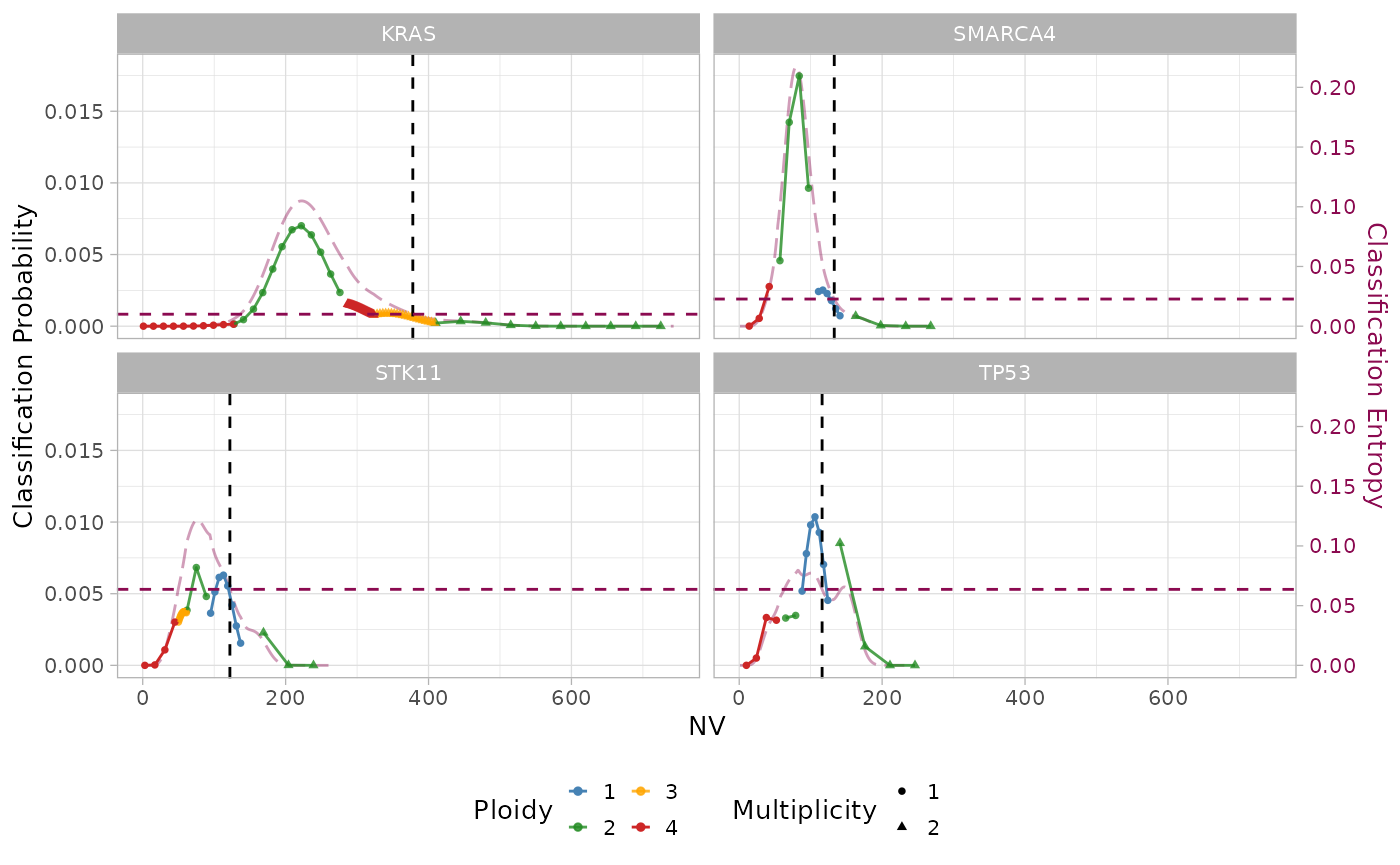
The shape parameters of the Beta distribution ensure that the mean and the variance correspond to the values we provided. The dashed line indicate the input purity estimate, used as the mean of the distribution.

We are now ready to run the classification step through function classify, using the priors we obtained for $(k,m)$ configurations, read count rate per chromosome copy $\eta$ and sample purity $\pi$ . We must provide the number of CPU cores num_cores we want to use for the parallel MCMC sampling chains, as well as the number of iterations for the warm-up (iter_warmup) and the proper sampling (iter_sampling) steps. We also must specify paths for the directories where we want to store the results (results_dir), the stan fit objects (stan_fit_dir) in case we want to store them (stan_fit_dump = TRUE) and, in case we want to generate a reporting summary plot (generate_report_plot = TRUE), the directory where to store the images (reports_dir).

out = classify(
  x = x,
  k_max = 8,
  priors_k_m = priors_pcawg_hmf,
  priors_eta = priors_eta,
  purity_error = 0.05,
  num_cores = 4,
  iter_warmup = 1000,
  iter_sampling = 2000,
  num_chains = 4,
  results_dir = '~/INCOMMON_inference/results',
  generate_report_plot = FALSE,
  reports_dir = '~/INCOMMON_inference/reports',
  stan_fit_dump = FALSE,
  stan_fit_dir = '~/INCOMMON_results/stan_fits/'
)

print(out)
#> ── [ INCOMMON ]  175054 PASS mutations across 24018 samples, with 290 mutant gen
#> ℹ Average sample purity: 0.4
#> ℹ Average sequencing depth: 649
#> # A tibble: 4 × 36
#>   sample    tumor_type purity purity_map eta_map chr     from     to gene  ref  
#>   <chr>     <chr>       <dbl>      <dbl>   <dbl> <chr>  <dbl>  <dbl> <chr> <chr>
#> 1 P-0002081 LUAD          0.6      0.639    188. chr12 2.54e7 2.54e7 KRAS  C    
#> 2 P-0002081 LUAD          0.6      0.639    188. chr17 7.58e6 7.58e6 TP53  G    
#> 3 P-0002081 LUAD          0.6      0.639    188. chr19 1.22e6 1.22e6 STK11 C    
#> 4 P-0002081 LUAD          0.6      0.639    188. chr19 1.11e7 1.11e7 SMAR… -    
#> # ℹ 26 more variables: alt <chr>, NV <int>, DP <int>, VAF <dbl>, map_k <int>,
#> #   map_m <int>, gene_role <chr>, OS_MONTHS <dbl>, OS_STATUS <dbl>,
#> #   SAMPLE_TYPE <chr>, MET_COUNT <dbl>, METASTATIC_SITE <chr>,
#> #   MET_SITE_COUNT <dbl>, PRIMARY_SITE <chr>, SUBTYPE_ABBREVIATION <chr>,
#> #   GENE_PANEL <chr>, SEX <chr>, TMB_NONSYNONYMOUS <dbl>, FGA <dbl>,
#> #   AGE_AT_SEQUENCING <dbl>, RACE <chr>, bayes_p_purity <dbl>,
#> #   bayes_p_eta <dbl>, post_pred_p.value_DP <dbl>, …

The output contains the maximum-a-posteriori (MAP) values of sample purity (purity_map), which is close to the input value (0.578 vs 0.6), read count rate per chromosome copy (eta_map) around 163, total copy number (map_k) and multiplicity (map_m).

The only mutant oncogene in the sample is KRAS, that is found in 8 copies, 5 of which mutated, whereas all the TSGs (TP53, SMARCA4, STK11) are in LOH, with only 1 mutant copy and total loss of the WT allele. These inferred values are consistent with the read counts with and without the variant and the estimated proportions of normal and tumour cells in the sample.

2.3 Visualising INCOMMON inference

Since INCOMMON is a Bayesian method, it provides more than point estimates for the quantities it infers. Instead, a full posterior distribution is evaluated.

For example, here we visualise the posterior distribution of copy number and multiplicity for the 4 mutant genes found in the analysed sample, using the function plot_posterior_k_m.

plot_posterior_k_m(x = out, k_max = out$parameters$k_max, z_km = out$input$z_km)

For KRAS, most of the probability mass is located at configurations of high total copy number with gain of the mutant allele. Conversely for the TSGs SMARCA4, STK11 and TP53, the posterior probability tends to accumulate on configurations of low total copy number with loss of the WT allele. The red markers indicate the MAP values reported in the above section.