1. Prior distribution of INCOMMON classes from PCAWG • INCOMMON

library(INCOMMON)
#> Warning: replacing previous import 'cli::num_ansi_colors' by
#> 'crayon::num_ansi_colors' when loading 'INCOMMON'
library(dplyr)
library(DT)

The inference of copy number and multiplicity of a mutation from read counts only can be much of a hard task, especially in cases where the sample purity $\pi$ or the sequencing depth $DP$ at the mutation site are low.

For this reason, INCOMMON allows using a prior distribution to improve classifications.

1.1 Empirical priors from PCAWG

When classifying mutations on a specific gene and in samples of a specific tumour type, a categorical prior distribution $p\left(z_{m,p}=1\right)=p_{m,p}$ , where $p$ is the ploidy and $m$ the mutation multiplicity, can be used to obtain more confident classifications, given that the prior probability of each class $p_{m,p}$ is obtained from reliable copy number calls. By default, INCOMMON relies on prior probability obtained from PCAWG whole genomes. From a set of high-confidence copy number calls validated by quality control, we obtained $p_{m,p}$ for each gene as the frequency of the corresponding INCOMMON class.

data("pcawg_priors")

The empirical priors from PCAWG are provided as an internal data table pcawg_priors and have the following format

where label represents the lower-level INCOMMON class in the format <p> N (Mutated: <m> N) and p is the corresponding value of $p_{m,p}$ .

1.1.1 Tumour-specific priors

If a gene was mutated in at least 5% of the samples from a tumour type, and at least in 20 samples, we built a tumour-specific prior. It is the case, for instance, of KRAS in pancreatic adenocarcinoma:

1.1.2 Pan-cancer priors

In cases where the requirements for a tumour-specific prior were not satisified, we pooled from all tumour types a pan-cancer prior. In the pcawg_priors table, these priors are identified by tumor_type equal to ‘PANCA’, meaning pan-cancer.

1.2 User-defined priors

The user who may want to leverage priors obtained in a different way (e.g. from other datasets or for a specific gene or tumour type not included in pcawg_priors), can easily do that by creating a similar data table.

For example:

my_priors = tibble(gene = 'my_gene',
                   tumor_type = 'my_tumor_type', 
                   label = c("1N (Mutated: 1N)",
                             "2N (Mutated: 1N)",
                             "2N (Mutated: 2N)",
                             "3N (Mutated: 1N)",
                             "3N (Mutated: 2N)",
                             "4N (Mutated: 1N)",
                             "4N (Mutated: 2N)"), 
                   p = c(0.2,0.3,0.1,0.1,0.1,0.1,0.1))

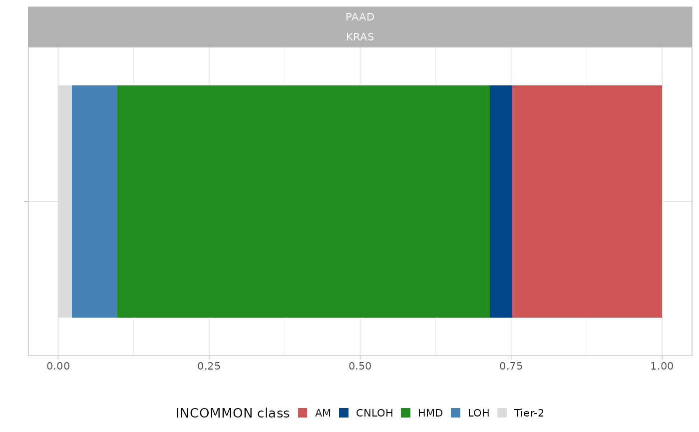
The only requirement is that the probabilities sum up to one $\sum\limits_{p=1}^4 \sum\limits_{m\leq p}p_{m,p}=1$ .

1.3 Visualising priors

The prior distribution used in a fit can be visualised a posteriori using the internal plotting function plot_prior. We can plot the prior distribution specific to a gene and tumour type used in the example classified MSK-MET data.

For example:

data("MSK_classified")
plot_prior(x = MSK_classified, 
           gene = 'KRAS',
           tumor_type = 'PAAD')
#> ✔ Loading CNAqc, 'Copy Number Alteration quality check'. Support : <https://caravagn.github.io/CNAqc/>