1. Prior distribution of mutation copy number and multiplicity from PCAWG • INCOMMON

library(INCOMMON)
#> Warning: replacing previous import 'cli::num_ansi_colors' by
#> 'crayon::num_ansi_colors' when loading 'INCOMMON'
library(dplyr)
library(DT)

The inference of copy number and multiplicity of a mutation from read counts only can be much of a hard task, especially in cases where the sample purity $\pi$ or the sequencing depth $DP$ at the mutation site are low.

For this reason, INCOMMON allows using a prior distribution to improve classifications.

1.1 Empirical priors from PCAWG

For the inference of mutation copy number and multiplicity on a specific gene and in samples of a specific tumour type, a Dirichlet prior distribution $p\left(k,m\right)=p_{k,m}$ , where $k$ is the total copy number and $m$ the mutation multiplicity, can be used to obtain more confident predictions, given that $p_{k,m}$ is obtained from reliable copy number calls. By default, INCOMMON relies on prior probability obtained from PCAWG and HMF whole genomes. From a set of high-confidence copy number calls validated by quality control, we obtained $p_{k,m}$ for each gene as the frequency of the corresponding INCOMMON class.

data("priors_pcawg_hmf")

The empirical priors from PCAWG and HMF are provided as an internal data table priors_pcawg_hmf and have the following format

#> Warning in instance$preRenderHook(instance): It seems your data is too big for
#> client-side DataTables. You may consider server-side processing:
#> https://rstudio.github.io/DT/server.html

where, for each gene and tumour_type, N represents the total counts in the used dataset, n is the count for the specific combination of k and m.

1.1.1 Tumour-specific priors

If a gene was mutated in at least 5% of the samples from a tumour type, and at least in 10 samples, we built a tumour-specific prior. It is the case, for instance, of KRAS in pancreatic adenocarcinoma (PAAD):

1.1.2 Pan-cancer priors

In cases where the requirements for a tumour-specific prior were not satisified, we pooled from all tumour types a pan-cancer prior. In the priors_pcawg_hmf table, these priors are identified by tumor_type equal to ‘PANCA’, meaning pan-cancer.

1.2 User-defined priors

The user who may want to leverage priors obtained in a different way (e.g. from other datasets or for a specific gene or tumour type not included in priors_pcawg_hmf), can easily do that by creating a similar data table.

For example:

my_priors = expand.grid(k=1:8, m = 1:8) %>% 
  dplyr::mutate(
    gene = 'my_gene',
    tumor_type = 'my_tumor_type') %>% 
  dplyr::filter(m<=k)

my_priors$n = rnorm(n = nrow(my_priors), mean = 50, sd = 10)
my_priors$N = sum(my_priors$n)

The only requirement is that n is a positive number and N is the sum of the values of n for a gene and tumour type pair.

1.3 Visualising priors

The prior distribution used in a fit can be visualised a posteriori using the internal plotting function plot_prior. We can plot the prior distribution specific to a gene and tumour type used in the example classified MSK-MET data.

For example:

plot_prior(x = priors_pcawg_hmf, 
           gene = 'KRAS',
           tumor_type = 'PAAD')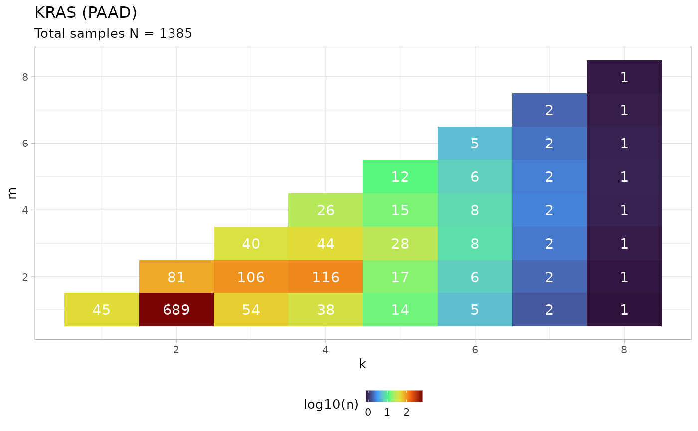

This example shows that, from the analysis of PCAWG and HMF datasets, KRAS mutations in pancreatic adenocarcinoma (PAAD) are most frequently found with $(k=2,m=1)$ configurations ( $N=689$ samples), i.e. in heterozygous diploid configurations. A relatively high frequency is also found for configurations with gain of the mutant copy: $(k=2,m=2)$ (CNLOH, $N=81$ samples), $(k=3,m=2)$ (mutant gain in trisomy, $N=106$ samples) and $(k=3,m=2)$ (mutant gain in tetrasomy, $N=116$ samples).