devil statistical model, CPU and GPU implementation

library(devil)
library(ggplot2)
library(dplyr)
library(tidyr)

Introduction

The devil package implements negative binomial regression for count data, particularly designed for single-cell RNA-seq analysis. This vignette explains:

1. The statistical model and fitting procedure
2. Shared computational steps (CPU and GPU)
3. CPU implementation with practical examples
4. GPU implementation (conceptual overview)
5. When to use CPU vs GPU
6. Performance optimization strategies

The Statistical Model

Devil fits a negative binomial generalized linear model for each gene:

$$Y_{ij} \sim \text{NB}(\mu_{ij}, \theta_i)$$

where:

• $Y_{ij}$ is the count for gene $i$ in cell $j$
• $\mu_{ij} = s_j \exp(\mathbf{X}_j^T \boldsymbol{\beta}_i)$ is the expected count
• $s_j$ is the size factor for cell $j$ (normalization)
• $\mathbf{X}_j$ is the design matrix row for cell $j$ (covariates)
• $\boldsymbol{\beta}_i$ is the coefficient vector for gene $i$
• $\theta_i$ is the overdispersion parameter for gene $i$

The model accounts for:

• Technical variation via size factors
• Biological covariates via the design matrix
• Overdispersion beyond Poisson variation

Common Steps (CPU and GPU)

Both implementations share the following preprocessing steps:

1. Size Factor Calculation

Size factors normalize for differences in sequencing depth across cells.

# Simulate example data
set.seed(123)
n_genes <- 500
n_cells <- 200
counts <- matrix(
    rnbinom(n_genes * n_cells, mu = 20, size = 5),
    nrow = n_genes, ncol = n_cells
)
rownames(counts) <- paste0("Gene", seq_len(n_genes))
colnames(counts) <- paste0("Cell", seq_len(n_cells))

# Create design matrix (two groups)
group <- factor(rep(c("Control", "Treatment"), each = n_cells/2))
design <- model.matrix(~ group)

Available normalization methods:

# Method 1: Geometric mean normalization (default, fast)
fit_normed <- fit_devil(
    input_matrix = counts,
    design_matrix = design,
    size_factors = "normed_sum",
    verbose = FALSE
)

# Method 2: Psi-normalization (robust to highly variable genes)
fit_psi <- fit_devil(
    input_matrix = counts,
    design_matrix = design,
    size_factors = "psinorm",
    verbose = FALSE
)

# Method 3: No normalization (all size factors = 1)
fit_no_norm <- fit_devil(
    input_matrix = counts,
    design_matrix = design,
    size_factors = NULL,
    verbose = FALSE
)

# Compare size factors
sf_comparison <- data.frame(
    cell = seq_len(n_cells),
    normed_sum = fit_normed$size_factors,
    psinorm = fit_psi$size_factors,
    no_norm = fit_no_norm$size_factors
)

sf_comparison %>%
    pivot_longer(-cell, names_to = "method", values_to = "size_factor") %>%
    ggplot(aes(x = cell, y = size_factor, color = method)) +
    geom_line() +
    theme_bw() +
    labs(title = "Size factors across normalization methods",
         x = "Cell index", y = "Size factor")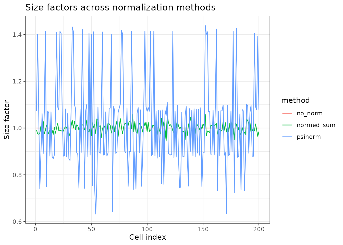

Interpretation:

• normed_sum: Fast, works for most datasets
• psinorm: More robust when many genes are highly variable
• NULL: Use when data is already normalized

2. Offset Vector Computation

The offset vector incorporates size factors into the model:

# The offset is computed as: log(size_factor) + offset_constant
offset_constant <- 0  # default
offset_vector <- log(fit_normed$size_factors) + offset_constant

# Visualize the relationship
data.frame(
    size_factor = fit_normed$size_factors,
    offset = fit_normed$offset_vector
) %>%
    ggplot(aes(x = size_factor, y = offset)) +
    geom_point(alpha = 0.5) +
    geom_smooth(method = "lm", se = FALSE, color = "red") +
    theme_bw() +
    labs(title = "Relationship between size factors and offsets",
         x = "Size factor", y = "Offset (log scale)")
#> `geom_smooth()` using formula = 'y ~ x'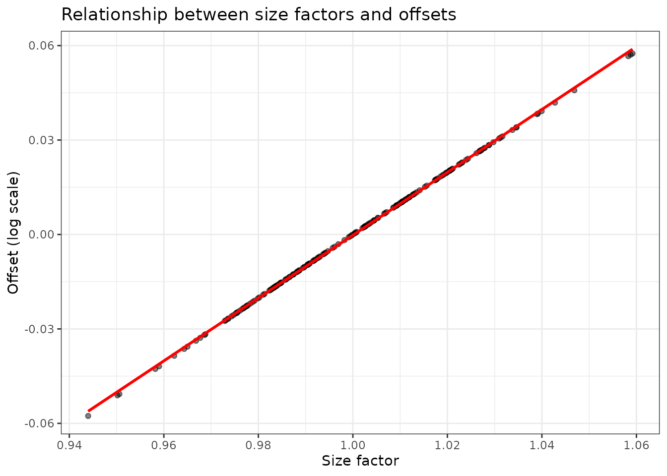

CPU Implementation

The CPU implementation processes genes in parallel using multiple cores.

Workflow Overview

1. Initialize overdispersion parameters (θ)
   ├─ If init_overdispersion = NULL: estimate from data
   └─ Otherwise: use provided value
   
2. Initialize beta coefficients (β)
   ├─ If init_beta_rough = TRUE: simple log-mean initialization
   └─ Otherwise: proper GLM initialization
   
3. Fit beta coefficients (parallel across genes)
   
4. Fit overdispersion parameters (parallel across genes)
   ├─ "MOM": Method of moments (fast, non-iterative)
   └─ "old"/"MLE": Maximum likelihood with Cox-Reid adjustment

CPU Example with Detailed Timing

# Small dataset for demonstration
set.seed(456)

n_genes_small <- 50
n_cells_small <- 10000

# Gene-specific baseline expression (log-normal is realistic for RNA-seq)
gene_means <- rlnorm(
  n_genes_small,
  meanlog = log(15),
  sdlog   = 0.8
)

# Gene-specific overdispersion (theta)
gene_theta <- rlnorm(
  n_genes_small,
  meanlog = log(3),
  sdlog   = 0.7
)

counts_small <- matrix(
  0,
  nrow = n_genes_small,
  ncol = n_cells_small
)

for (g in seq_len(n_genes_small)) {
  counts_small[g, ] <- rnbinom(
    n_cells_small,
    mu   = gene_means[g],
    size = gene_theta[g]
  )
}

rownames(counts_small) <- paste0("Gene", seq_len(n_genes_small))
colnames(counts_small) <- paste0("Cell", seq_len(n_cells_small))

# Two-group design
design_small <- model.matrix(
  ~ factor(rep(c("Control", "Treatment"), each = n_cells_small / 2))
)

# CPU fit with different overdispersion strategies
system.time({
    fit_cpu_mom <- fit_devil(
        input_matrix = counts_small,
        design_matrix = design_small,
        size_factors = "normed_sum",
        overdispersion = "MOM",
        parallel.cores = 1,
        verbose = TRUE
    )
})
#> Compute size factors
#> Calculating size factors using method: normed_sum
#> Size factors calculated successfully.
#> Range: [0.6759, 1.6736]
#> Initialize theta
#> Initialize beta
#> Fitting beta coefficients
#> Fit overdispersion (mode = MOM)
#>    user  system elapsed 
#>   0.119   0.195   0.098

system.time({
    fit_cpu_new <- fit_devil(
        input_matrix = counts_small,
        design_matrix = design_small,
        size_factors = "normed_sum",
        overdispersion = "MLE",
        parallel.cores = 1,
        verbose = TRUE
    )
})
#> Compute size factors
#> Calculating size factors using method: normed_sum
#> Size factors calculated successfully.
#> Range: [0.6759, 1.6736]
#> Initialize theta
#> Initialize beta
#> Fitting beta coefficients
#> Fit overdispersion (mode = MLE)
#>    user  system elapsed 
#>   0.314   0.638   0.253

Examining Iteration Counts

# Beta fitting iterations (per gene)
beta_iter_summary <- data.frame(
    iterations = fit_cpu_new$iterations$beta_iters
)

ggplot(beta_iter_summary, aes(x = iterations)) +
    geom_histogram(bins = 20, fill = "steelblue", alpha = 0.7) +
    theme_bw() +
    labs(title = "Beta coefficient fitting: iterations per gene",
         x = "Number of iterations", y = "Number of genes")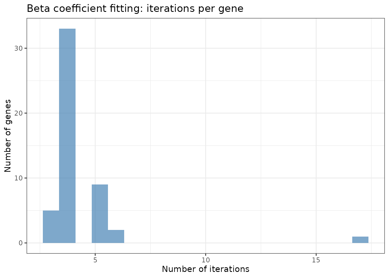

# Theta fitting iterations (per gene)
if (!is.na(fit_cpu_new$iterations$theta_iters[1])) {
    theta_iter_summary <- data.frame(
        iterations = fit_cpu_new$iterations$theta_iters
    )
    
    ggplot(theta_iter_summary, aes(x = iterations)) +
        geom_histogram(bins = 20, fill = "coral", alpha = 0.7) +
        theme_bw() +
        labs(title = "Overdispersion fitting: iterations per gene",
             x = "Number of iterations", y = "Number of genes")
}

Overdispersion Estimation Strategies

The CPU implementation offers three strategies for estimating overdispersion:

1. Method of Moments (MOM) - Fastest

fit_mom <- fit_devil(
    input_matrix = counts_small,
    design_matrix = design_small,
    overdispersion = "MOM",
    verbose = FALSE
)

# MOM is non-iterative (0 iterations)
print(paste("Theta iterations (MOM):", unique(fit_mom$iterations$theta_iters)))
#> [1] "Theta iterations (MOM): 0"

When to use:
Large datasets or GPU-based workflows, when speed and scalability are critical and a fully iterative dispersion fit is impractical.

How it works:
In a regression setting, MOM does not rely on the raw sample mean and variance of counts. Instead, it estimates overdispersion from the residual variability around the fitted mean $\mu_{ij}$ implied by the design matrix and offsets.

Concretely, after fitting (or updating) the regression coefficients $\boldsymbol{\beta}_i$, devil computes fitted means $\mu_{ij}$ and matches the negative binomial mean–variance relationship $$\mathrm{Var}(Y_{ij}) = \mu_{ij} + \frac{\mu_{ij}^2}{\theta_i}$$ using squared residuals $(y_{ij}-\mu_{ij})^2$ to obtain a closed-form, non-iterative estimate of $\theta_i$.

This makes MOM extremely fast and well suited for large-scale single-cell analyses, while still accounting for the effects of covariates and normalization through $\mu_{ij}$.

2. MLE with Cox-Reid (MLE) - Most Accurate

fit_mle <- fit_devil(
    input_matrix = counts_small,
    design_matrix = design_small,
    overdispersion = "old",
    max_iter = 200,
    verbose = FALSE
)

When to use: Maximum precision, small datasets. How it works: Maximum likelihood estimation with Cox-Reid adjustment.

Comparing Overdispersion Estimates

theta_comparison <- data.frame(
    gene = seq_len(n_genes_small),
    MOM = fit_mom$overdispersion,
    MLE = fit_mle$overdispersion
)

theta_comparison %>%
    #pivot_longer(-gene, names_to = "method", values_to = "theta") %>%
    ggplot(aes(x = log10(MOM), y = log10(MLE))) +
    geom_point() +
    theme_bw() +
    labs(title = "Overdispersion estimates across methods",
         x = "log10(θ MOM)", y = "log10(θ MLE)")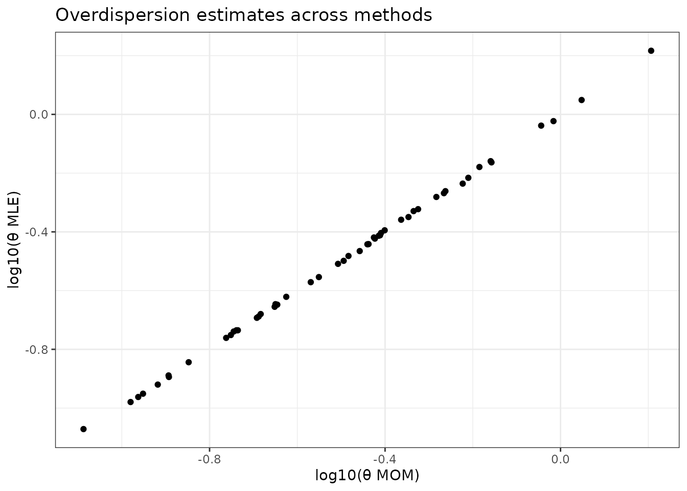

# Correlation between methods
cor(theta_comparison[, -1]) %>% round(3)
#>     MOM MLE
#> MOM   1   1
#> MLE   1   1

Interpretation: Methods generally agree, but MLE may provide more stable estimates for difficult genes. MOM is fastest but may be less precise for genes with extreme overdispersion.

Beta Initialization Strategies

# Compare initialization strategies
time_rough <- system.time({
    fit_rough <- fit_devil(
        input_matrix = counts_small,
        design_matrix = design_small,
        init_beta_rough = TRUE,
        verbose = FALSE
    )
})

time_proper <- system.time({
    fit_proper <- fit_devil(
        input_matrix = counts_small,
        design_matrix = design_small,
        init_beta_rough = FALSE,
        verbose = FALSE
    )
})

print(paste("Rough init:", round(time_rough["elapsed"], 2), "sec"))
#> [1] "Rough init: 0.05 sec"
print(paste("Proper init:", round(time_proper["elapsed"], 2), "sec"))
#> [1] "Proper init: 0.09 sec"

# Check if results are similar
cor(fit_rough$beta[, 2], fit_proper$beta[, 2])
#> [1] 0.9999904

Recommendation: - init_beta_rough = FALSE (default): Proper GLM initialization, more robust - init_beta_rough = TRUE: Faster for very large datasets

The rough initialization simply uses log(mean(y) + 1) for the intercept and zeros for other coefficients. The proper initialization fits a simplified GLM to get better starting values.

GPU Implementation (Conceptual)

The GPU implementation uses CUDA for massive parallelization across genes.

GPU Workflow

1. Compute size factors and offsets (same as CPU)
   └─ This preprocessing happens on CPU

2. Batch genes for memory efficiency
   ├─ Genes are divided into batches of size 'batch_size'
   └─ Default: 1024 genes per batch

3. GPU kernel: Fit beta coefficients
   ├─ Each GPU thread handles one gene
   ├─ Thousands of genes fitted simultaneously
   └─ Iterative weighted least squares on GPU

4. Overdispersion: Method of Moments only
   ├─ Computed on GPU (non-iterative)
   └─ Fast calculation across all genes

Key Differences from CPU

Feature	CPU	GPU
Parallelization	Across genes using CPU cores (typically 4-64)	Across genes using GPU threads (thousands)
Memory model	Distributed (per core)	Shared (batched on GPU memory)
Overdispersion	MOM, Iterative, or MLE	MOM only
Beta initialization	Full initialization available	Simplified initialization
Batch processing	All genes or chunked by core	Always batched for GPU memory
Best for	Small-medium datasets (<5k genes)	Large datasets (>10k genes, >5k cells)
Setup	Works out of the box	Requires CUDA toolkit and recompilation