Getting Started with devil:
Differential Expression Analysis in scRNA-seq
Source: vignettes/articles/Introduction.Rmd
Introduction.RmdThis tutorial guides you through the use of the devil
package for analyzing differential gene expression in single-cell RNA
sequencing (scRNA-seq) data.
Prerequisites
Before we begin, make sure you have the required packages installed
library(devil)
library(scRNAseq)
#> Loading required package: SingleCellExperiment
#> Loading required package: SummarizedExperiment
#> Loading required package: MatrixGenerics
#> Loading required package: matrixStats
#>
#> Attaching package: 'MatrixGenerics'
#> The following objects are masked from 'package:matrixStats':
#>
#>     colAlls, colAnyNAs, colAnys, colAvgsPerRowSet, colCollapse,
#>     colCounts, colCummaxs, colCummins, colCumprods, colCumsums,
#>     colDiffs, colIQRDiffs, colIQRs, colLogSumExps, colMadDiffs,
#>     colMads, colMaxs, colMeans2, colMedians, colMins, colOrderStats,
#>     colProds, colQuantiles, colRanges, colRanks, colSdDiffs, colSds,
#>     colSums2, colTabulates, colVarDiffs, colVars, colWeightedMads,
#>     colWeightedMeans, colWeightedMedians, colWeightedSds,
#>     colWeightedVars, rowAlls, rowAnyNAs, rowAnys, rowAvgsPerColSet,
#>     rowCollapse, rowCounts, rowCummaxs, rowCummins, rowCumprods,
#>     rowCumsums, rowDiffs, rowIQRDiffs, rowIQRs, rowLogSumExps,
#>     rowMadDiffs, rowMads, rowMaxs, rowMeans2, rowMedians, rowMins,
#>     rowOrderStats, rowProds, rowQuantiles, rowRanges, rowRanks,
#>     rowSdDiffs, rowSds, rowSums2, rowTabulates, rowVarDiffs, rowVars,
#>     rowWeightedMads, rowWeightedMeans, rowWeightedMedians,
#>     rowWeightedSds, rowWeightedVars
#> Loading required package: GenomicRanges
#> Loading required package: stats4
#> Loading required package: BiocGenerics
#>
#> Attaching package: 'BiocGenerics'
#> The following objects are masked from 'package:stats':
#>
#>     IQR, mad, sd, var, xtabs
#> The following objects are masked from 'package:base':
#>
#>     anyDuplicated, aperm, append, as.data.frame, basename, cbind,
#>     colnames, dirname, do.call, duplicated, eval, evalq, Filter, Find,
#>     get, grep, grepl, intersect, is.unsorted, lapply, Map, mapply,
#>     match, mget, order, paste, pmax, pmax.int, pmin, pmin.int,
#>     Position, rank, rbind, Reduce, rownames, sapply, saveRDS, setdiff,
#>     table, tapply, union, unique, unsplit, which.max, which.min
#> Loading required package: S4Vectors
#>
#> Attaching package: 'S4Vectors'
#> The following object is masked from 'package:utils':
#>
#>     findMatches
#> The following objects are masked from 'package:base':
#>
#>     expand.grid, I, unname
#> Loading required package: IRanges
#> Loading required package: GenomeInfoDb
#> Loading required package: Biobase
#> Welcome to Bioconductor
#>
#>     Vignettes contain introductory material; view with
#>     'browseVignettes()'. To cite Bioconductor, see
#>     'citation("Biobase")', and for packages 'citation("pkgname")'.
#>
#> Attaching package: 'Biobase'
#> The following object is masked from 'package:MatrixGenerics':
#>
#>     rowMedians
#> The following objects are masked from 'package:matrixStats':
#>
#>     anyMissing, rowMedians
#> Warning: replacing previous import 'S4Arrays::makeNindexFromArrayViewport' by
#> 'DelayedArray::makeNindexFromArrayViewport' when loading 'SummarizedExperiment'
#> Warning: replacing previous import 'S4Arrays::makeNindexFromArrayViewport' by
#> 'DelayedArray::makeNindexFromArrayViewport' when loading 'HDF5Array'
Loading and preparing your data
Let’s start by loading a sample dataset from the
scRNAseq package
# Load the example dataset
data <- scRNAseq::BaronPancreasData()

# Extract counts and metadata
counts <- data@assays@data[[1]]
metadata <- data@colData

# Display dataset dimensions
cat("Number of genes:", nrow(counts), "\n")
#> Number of genes: 20125
cat("Number of cells:", ncol(counts), "\n")
#> Number of cells: 8569
cat("Metadata features:", ncol(metadata), "\n")
#> Metadata features: 2
Data cleaning
Filtering cell types
To focus our analysis, we retain only the three most abundant cell types.
# Select the three most expressed cell types
top_3_ct <- names(sort(table(metadata$label), decreasing = TRUE)[1:3])
cell_filter <- metadata$label %in% top_3_ct
metadata <- metadata[cell_filter,]
counts <- counts[, cell_filter]

cat("Remaining cells after filtering:", nrow(metadata), "\n")
#> Remaining cells after filtering: 5928Setting up the Design matrix
The design matrix specifies the experimental conditions for each cell:
# Create design matrix based on biological conditions
design_matrix <- model.matrix(~label, data = metadata)

# View unique conditions in your data
print(unique(metadata$label))
#> [1] "beta"   "ductal" "alpha"
Model fitting
Next, we fit the statistical model to the filtered dataset using the
devil::fit_devil() function.
Testing for Differential Expression
Understanding Contrast Vectors
In order to test the data you need to specify your null hypothesis using a contrast vector . Considering a gene along with its inferred coefficient , the null hypothesis is usually defined as
For example, if you are interested in the genes that are differentially expressed between the “beta” and “ductal” cell types, you need to find the genes for which we strongly reject the null hypothesis
$$ \beta_{beta} = \beta_{ductal} \hspace{5mm} \rightarrow \hspace{5mm} \beta_{beta} - \beta_{ductal} = 0$$
which is equivalent to defining the contrast vector
.
Once the contrast vector is defined, you can test the null hypothesis
using the test_de function.
# Test differential expression between conditions
contrast <- c(0, 1, -1)
test_results <- devil::test_de(fit, contrast, max_lfc = 20)

# Add gene names if missing
if (!('name' %in% colnames(test_results))) {
  test_results$name <- as.character(1:nrow(test_results))
}
The test results include:
-
pval: raw p-value -
adj_pval: adjusted p-value (corrected for multiple testing) -
lfc: log2 fold change between conditions
Visualizing Results
Create a volcano plot to visualize significant genes
devil::plot_volcano(
  test_results,
  lfc_cut = 1,          # Log fold-change cutoff
  pval_cut = 0.05,      # P-value significance threshold
  labels = TRUE,        # Show gene labels
  point_size = 2
)
#> 82 genes have adjusted p-value equal to 0, will be set to 1.3394613724402e-319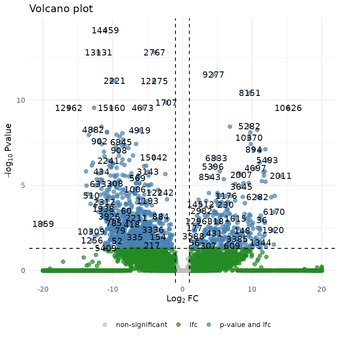
Conclusion
In this tutorial, we covered the essential workflow for differential expression analysis using the devil package, including:
- Loading and preprocessing scRNA-seq data
- Filtering low-quality genes and selecting cell types
- Constructing a design matrix for statistical modeling
- Fitting the devil model and testing for differential expression
- Visualizing significant results with a volcano plot