devil is an R package for differential expression
analysis in single-cell RNA sequencing (scRNA-seq) data. It supports
both single- and multi-patient experimental designs, implementing robust
statistical methods to identify differentially expressed genes while
accounting for technical and biological variability.
Key features are:
- Flexible experimental design support (single/multiple patients)
- Robust statistical testing framework
- Efficient implementation for large-scale datasets
Installation
You can install the current version of devil from GitHub with:
devtools::install_github("caravagnalab/devil")Example
This tutorial walks through a minimal, end-to-end workflow for
differential expression (DE) with devil on
a public scRNA-seq dataset. You will: (1) load data, (2) filter
cells/genes, (3) build a design, (4) fit the model, (5) specify
contrasts, and (6) visualize results.
If your study has multiple patients/donors, devil can
compute clustered (patient-aware) standard errors via a
cluster argument.
Prerequisites
# If needed:
# install.packages("BiocManager")
# BiocManager::install(c("scRNAseq","SingleCellExperiment"))

library(devil)
library(scRNAseq)
#> Loading required package: SingleCellExperiment
#> Loading required package: SummarizedExperiment
#> Loading required package: MatrixGenerics
#> Loading required package: matrixStats
#>
#> Attaching package: 'MatrixGenerics'
#> The following objects are masked from 'package:matrixStats':
#>
#>     colAlls, colAnyNAs, colAnys, colAvgsPerRowSet, colCollapse,
#>     colCounts, colCummaxs, colCummins, colCumprods, colCumsums,
#>     colDiffs, colIQRDiffs, colIQRs, colLogSumExps, colMadDiffs,
#>     colMads, colMaxs, colMeans2, colMedians, colMins, colOrderStats,
#>     colProds, colQuantiles, colRanges, colRanks, colSdDiffs, colSds,
#>     colSums2, colTabulates, colVarDiffs, colVars, colWeightedMads,
#>     colWeightedMeans, colWeightedMedians, colWeightedSds,
#>     colWeightedVars, rowAlls, rowAnyNAs, rowAnys, rowAvgsPerColSet,
#>     rowCollapse, rowCounts, rowCummaxs, rowCummins, rowCumprods,
#>     rowCumsums, rowDiffs, rowIQRDiffs, rowIQRs, rowLogSumExps,
#>     rowMadDiffs, rowMads, rowMaxs, rowMeans2, rowMedians, rowMins,
#>     rowOrderStats, rowProds, rowQuantiles, rowRanges, rowRanks,
#>     rowSdDiffs, rowSds, rowSums2, rowTabulates, rowVarDiffs, rowVars,
#>     rowWeightedMads, rowWeightedMeans, rowWeightedMedians,
#>     rowWeightedSds, rowWeightedVars
#> Loading required package: GenomicRanges
#> Loading required package: stats4
#> Loading required package: BiocGenerics
#> Loading required package: generics
#>
#> Attaching package: 'generics'
#> The following objects are masked from 'package:base':
#>
#>     as.difftime, as.factor, as.ordered, intersect, is.element, setdiff,
#>     setequal, union
#>
#> Attaching package: 'BiocGenerics'
#> The following objects are masked from 'package:stats':
#>
#>     IQR, mad, sd, var, xtabs
#> The following objects are masked from 'package:base':
#>
#>     anyDuplicated, aperm, append, as.data.frame, basename, cbind,
#>     colnames, dirname, do.call, duplicated, eval, evalq, Filter, Find,
#>     get, grep, grepl, is.unsorted, lapply, Map, mapply, match, mget,
#>     order, paste, pmax, pmax.int, pmin, pmin.int, Position, rank,
#>     rbind, Reduce, rownames, sapply, saveRDS, table, tapply, unique,
#>     unsplit, which.max, which.min
#> Loading required package: S4Vectors
#>
#> Attaching package: 'S4Vectors'
#> The following object is masked from 'package:utils':
#>
#>     findMatches
#> The following objects are masked from 'package:base':
#>
#>     expand.grid, I, unname
#> Loading required package: IRanges
#> Loading required package: Seqinfo
#> Loading required package: Biobase
#> Welcome to Bioconductor
#>
#>     Vignettes contain introductory material; view with
#>     'browseVignettes()'. To cite Bioconductor, see
#>     'citation("Biobase")', and for packages 'citation("pkgname")'.
#>
#> Attaching package: 'Biobase'
#> The following object is masked from 'package:MatrixGenerics':
#>
#>     rowMedians
#> The following objects are masked from 'package:matrixStats':
#>
#>     anyMissing, rowMedians
library(SingleCellExperiment)
library(SummarizedExperiment)
library(Matrix)
#>
#> Attaching package: 'Matrix'
#> The following object is masked from 'package:S4Vectors':
#>
#>     expand
library(dplyr)
#>
#> Attaching package: 'dplyr'
#> The following object is masked from 'package:Biobase':
#>
#>     combine
#> The following objects are masked from 'package:GenomicRanges':
#>
#>     intersect, setdiff, union
#> The following object is masked from 'package:Seqinfo':
#>
#>     intersect
#> The following objects are masked from 'package:IRanges':
#>
#>     collapse, desc, intersect, setdiff, slice, union
#> The following objects are masked from 'package:S4Vectors':
#>
#>     first, intersect, rename, setdiff, setequal, union
#> The following objects are masked from 'package:BiocGenerics':
#>
#>     combine, intersect, setdiff, setequal, union
#> The following object is masked from 'package:generics':
#>
#>     explain
#> The following object is masked from 'package:matrixStats':
#>
#>     count
#> The following object is masked from 'package:devil':
#>
#>     group_data
#> The following objects are masked from 'package:stats':
#>
#>     filter, lag
#> The following objects are masked from 'package:base':
#>
#>     intersect, setdiff, setequal, union
Load and inspect data
We’ll use the Baron pancreas dataset from scRNAseq.
sce <- scRNAseq::BaronPancreasData() # SingleCellExperiment
sce
#> class: SingleCellExperiment
#> dim: 20125 8569
#> metadata(0):
#> assays(1): counts
#> rownames(20125): A1BG A1CF ... ZZZ3 pk
#> rowData names(0):
#> colnames(8569): human1_lib1.final_cell_0001 human1_lib1.final_cell_0002
#>   ... human4_lib3.final_cell_0700 human4_lib3.final_cell_0701
#> colData names(2): donor label
#> reducedDimNames(0):
#> mainExpName: NULL
#> altExpNames(0):
Extract counts and metadata using accessors:
counts <- SummarizedExperiment::assay(sce, "counts")
meta <- as.data.frame(SummarizedExperiment::colData(sce))

cat("Genes:", nrow(counts), "\nCells:", ncol(counts), "\n")
#> Genes: 20125
#> Cells: 8569
stopifnot("label" %in% colnames(meta))
head(meta$label)
#> [1] "acinar" "acinar" "acinar" "acinar" "acinar" "acinar"
Tip: If you have a patient/donor column (often
donor or patient), keep it, we’ll optionally
pass it to cluste= later.
Light filtering
Keep the three most abundant cell types; filter lowly expressed genes.
# keep 3 largest cell types
top3 <- names(sort(table(meta$label), decreasing = TRUE))[1:3]
keep_cells <- meta$label %in% top3
counts <- counts[, keep_cells, drop = FALSE]
meta <- meta[keep_cells, , drop = FALSE]

# gene filter: expressed (>=1 UMI) in >= 1% of kept cells
min_cells <- max(1, floor(0.01 * ncol(counts)))
keep_genes <- Matrix::rowSums(counts >= 1) >= min_cells
counts <- counts[keep_genes, , drop = FALSE]

cat("After filtering — Genes:", nrow(counts), "Cells:", ncol(counts), "\n")
#> After filtering — Genes: 11951 Cells: 5928
table(meta$label)
#>
#>  alpha   beta ductal
#>   2326   2525   1077
Optionally restrict to highly expressed genes for a faster demo (skip for real analyses):
Design matrix
Build a no-intercept design so each coefficient corresponds to a cell type.
meta$label <- droplevels(factor(meta$label))
design <- model.matrix(~ 0 + label, data = meta)
colnames(design) <- gsub("^label", "", colnames(design))
colnames(design)
#> [1] "alpha"  "beta"   "ductal"
(Optional) Cluster variable for patient-aware SEs, if available:
Fit the model
fit_devil() expects a counts matrix (genes × cells), a
design (cells × covariates). The parameters
size_factors="normed_sum" computes internally a size factor
that will scale expression based on the library size of each cell.
fit <- devil::fit_devil(
    x = as.matrix(counts),
    design_matrix = design,
    clusters = as.factor(clusters),
    overdispersion = "MOM",
    offset = 1e-6,
    init_overdispersion = NULL,
    size_factors = "normed_sum",

    verbose = TRUE,
    max_iter = 200,
    tolerance = 1e-4
)
#> Compute size factors
#> Calculating size factors using method: normed_sum
#> Size factors calculated successfully.
#> Range: [0.1036, 8.0148]
#> ==> Initializing parameters
#> Initialize theta
#> Initialize beta
#> Fitting expression coefficients and overdispersion
#> Aggregating results
Specify contrasts
With a no-intercept design, each column is a cell-type mean on the
log scale.
To test “beta vs ductal”, define the contrast
(+1 * beta) + (-1 * ductal) and zero elsewhere.
make_contrast <- function(design, from, to) {
    stopifnot(from %in% colnames(design), to %in% colnames(design))
    c <- rep(0, ncol(design))
    names(c) <- colnames(design)
    c[from] <- 1
    c[to] <- -1
    as.numeric(c)
}

contrast <- make_contrast(design, from = "beta", to = "ductal")
contrast
#> [1]  0  1 -1
If your labels differ, update from/to
accordingly—use colnames(design) to see available
levels.
Test for differential expression
Run a Wald test with optional clustered SEs if
cluster exists.
test <- devil::test_de(
    fit,
    contrast = contrast,
    max_lfc  = 10 # Cap extreme fold changes
)

# Add gene names if missing
if (!("name" %in% colnames(test))) {
    if (!is.null(rownames(counts))) {
        test$name <- rownames(counts)
    } else {
        test$name <- as.character(seq_len(nrow(test)))
    }
}
Quick peek at the top hits:
test %>%
    dplyr::arrange(adj_pval, desc(abs(lfc))) %>%
    dplyr::select(name, lfc, pval, adj_pval) %>%
    head(10)
#> # A tibble: 10 × 4
#>    name     lfc      pval  adj_pval
#>    <chr>  <dbl>     <dbl>     <dbl>
#>  1 ERO1B   4.44 8.59e-285 4.30e-282
#>  2 KRT7   -9.35 5.43e-212 1.36e-209
#>  3 CPE     4.40 9.64e-193 1.61e-190
#>  4 G6PC2   5.78 1.48e-185 1.85e-183
#>  5 HADH    3.32 6.28e-150 6.28e-148
#>  6 UCHL1   4.63 6.00e-149 5.00e-147
#>  7 CD24   -3.77 6.79e-136 4.85e-134
#>  8 PEMT    3.95 1.37e-126 8.55e-125
#>  9 PMEPA1 -7.03 1.63e-124 9.05e-123
#> 10 TMOD1   4.67 7.39e-122 3.69e-120
Visualize results
devil::plot_volcano(
    test,
    lfc_cut = 1,
    pval_cut = 0.05,
    labels = TRUE,
    point_size = 1.8,
    title = "beta vs ductal"
)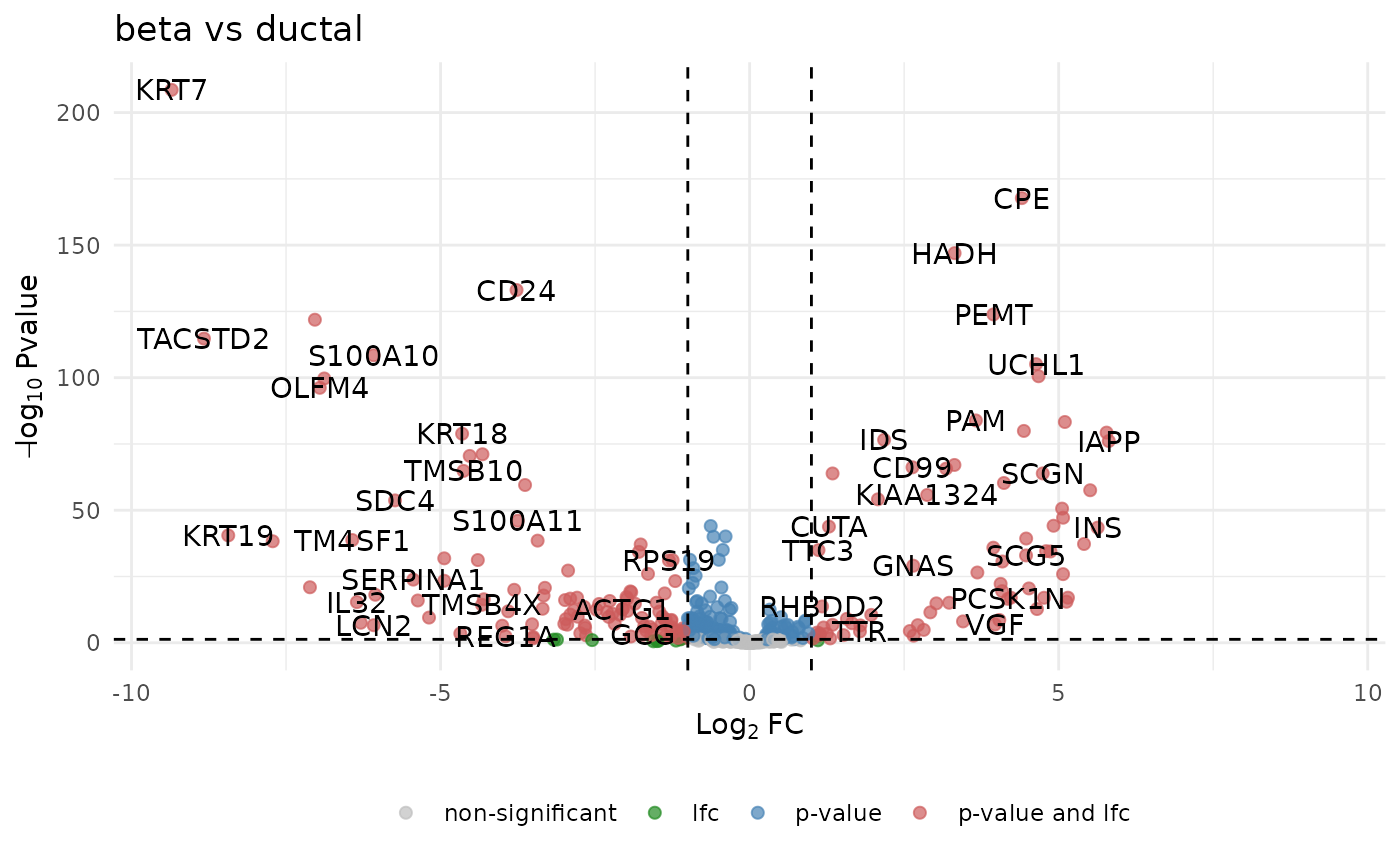
Volcano plot of DE genes
Session info
sessionInfo()
#> R version 4.6.0 (2026-04-24)
#> Platform: x86_64-pc-linux-gnu
#> Running under: Ubuntu 24.04.4 LTS
#>
#> Matrix products: default
#> BLAS:   /usr/lib/x86_64-linux-gnu/openblas-pthread/libblas.so.3
#> LAPACK: /usr/lib/x86_64-linux-gnu/openblas-pthread/libopenblasp-r0.3.26.so;  LAPACK version 3.12.0
#>
#> locale:
#>  [1] LC_CTYPE=C.UTF-8       LC_NUMERIC=C           LC_TIME=C.UTF-8
#>  [4] LC_COLLATE=C.UTF-8     LC_MONETARY=C.UTF-8    LC_MESSAGES=C.UTF-8
#>  [7] LC_PAPER=C.UTF-8       LC_NAME=C              LC_ADDRESS=C
#> [10] LC_TELEPHONE=C         LC_MEASUREMENT=C.UTF-8 LC_IDENTIFICATION=C
#>
#> time zone: UTC
#> tzcode source: system (glibc)
#>
#> attached base packages:
#> [1] stats4    stats     graphics  grDevices utils     datasets  methods
#> [8] base
#>
#> other attached packages:
#>  [1] dplyr_1.2.1                 Matrix_1.7-5
#>  [3] scRNAseq_2.26.0             SingleCellExperiment_1.34.0
#>  [5] SummarizedExperiment_1.42.0 Biobase_2.72.0
#>  [7] GenomicRanges_1.64.0        Seqinfo_1.2.0
#>  [9] IRanges_2.46.0              S4Vectors_0.50.1
#> [11] BiocGenerics_0.58.1         generics_0.1.4
#> [13] MatrixGenerics_1.24.0       matrixStats_1.5.0
#> [15] devil_0.99.0
#>
#> loaded via a namespace (and not attached):
#>   [1] DBI_1.3.0                 bitops_1.0-9
#>   [3] httr2_1.2.2               rlang_1.2.0
#>   [5] magrittr_2.0.5            otel_0.2.0
#>   [7] gypsum_1.8.0              compiler_4.6.0
#>   [9] RSQLite_3.53.1            DelayedMatrixStats_1.34.0
#>  [11] GenomicFeatures_1.64.0    png_0.1-9
#>  [13] systemfonts_1.3.2         vctrs_0.7.3
#>  [15] ProtGenerics_1.44.0       pkgconfig_2.0.3
#>  [17] crayon_1.5.3              fastmap_1.2.0
#>  [19] dbplyr_2.5.2              XVector_0.52.0
#>  [21] labeling_0.4.3            utf8_1.2.6
#>  [23] Rsamtools_2.28.0          rmarkdown_2.31
#>  [25] UCSC.utils_1.8.0          ragg_1.5.2
#>  [27] bit_4.6.0                 xfun_0.58
#>  [29] cachem_1.1.0              cigarillo_1.2.0
#>  [31] GenomeInfoDb_1.48.0       jsonlite_2.0.0
#>  [33] blob_1.3.0                rhdf5filters_1.24.0
#>  [35] DelayedArray_0.38.2       Rhdf5lib_2.0.0
#>  [37] BiocParallel_1.46.0       parallel_4.6.0
#>  [39] R6_2.6.1                  RColorBrewer_1.1-3
#>  [41] bslib_0.11.0              rtracklayer_1.72.0
#>  [43] jquerylib_0.1.4           Rcpp_1.1.1-1.1
#>  [45] knitr_1.51                tidyselect_1.2.1
#>  [47] abind_1.4-8               yaml_2.3.12
#>  [49] codetools_0.2-20          curl_7.1.0
#>  [51] lattice_0.22-9            alabaster.sce_1.12.0
#>  [53] tibble_3.3.1              S7_0.2.2
#>  [55] withr_3.0.2               KEGGREST_1.52.0
#>  [57] evaluate_1.0.5            desc_1.4.3
#>  [59] BiocFileCache_3.2.0       alabaster.schemas_1.12.0
#>  [61] ExperimentHub_3.2.0       Biostrings_2.80.1
#>  [63] pillar_1.11.1             BiocManager_1.30.27
#>  [65] filelock_1.0.3            RCurl_1.98-1.19
#>  [67] ggplot2_4.0.3             BiocVersion_3.23.1
#>  [69] ensembldb_2.36.1          scales_1.4.0
#>  [71] sparseMatrixStats_1.24.0  alabaster.base_1.12.0
#>  [73] alabaster.ranges_1.12.0   glue_1.8.1
#>  [75] alabaster.matrix_1.12.0   lazyeval_0.2.3
#>  [77] tools_4.6.0               AnnotationHub_4.2.0
#>  [79] BiocIO_1.22.0             GenomicAlignments_1.48.0
#>  [81] fs_2.1.0                  XML_3.99-0.23
#>  [83] rhdf5_2.56.0              grid_4.6.0
#>  [85] AnnotationDbi_1.74.0      HDF5Array_1.40.0
#>  [87] restfulr_0.0.16           cli_3.6.6
#>  [89] rappdirs_0.3.4            textshaping_1.0.5
#>  [91] S4Arrays_1.12.0           AnnotationFilter_1.36.0
#>  [93] gtable_0.3.6              alabaster.se_1.12.0
#>  [95] sass_0.4.10               digest_0.6.39
#>  [97] SparseArray_1.12.2        farver_2.1.2
#>  [99] rjson_0.2.23              memoise_2.0.1
#> [101] htmltools_0.5.9           pkgdown_2.2.0
#> [103] lifecycle_1.0.5           h5mread_1.4.0
#> [105] httr_1.4.8                bit64_4.8.2